
✨ Your Journey into the Magic of Integration ✨
Understanding Integration from Scratch – A Beginner’s Guide
🌟 Welcome to the World of Integration!
Welcome, dear learner! 😊 You’re about to embark on an exciting journey that will change the way you see the world around you. Integration isn’t just about numbers and formulas—it’s about understanding how things accumulate, grow, and come together to create something bigger. Whether you’re watching water fill a bathtub, calculating the total distance traveled on a road trip, or measuring the signal strength of your mobile phone across a city, integration is everywhere!
By the end of this chapter, you’ll not only understand what integration is, but you’ll also fall in love with its elegance and power. Let’s make math fun! 🎉
Chapter 1: 🔄 Derivatives vs. Integration – Two Sides of the Same Coin
1.1 What Are Derivatives? 📉
Think of derivatives as asking: “How fast is something changing right now?” It’s like checking your car’s speedometer.
Real-Life Example:
Imagine you’re driving on a highway. Your car’s speedometer shows 60 mph at this exact moment. That’s a derivative! It tells you your instantaneous rate of change of position with respect to time. 🚗💨
Mathematical notation: If your position is s(t), then velocity v(t) = ds/dt
1.2 What Is Integration? 📈
Integration asks the opposite question: “If I know how fast something is changing, what is the total accumulation?” It’s like figuring out the total distance you traveled on that road trip.
Real-Life Example:
You drove at 60 mph for 2 hours. How far did you travel? Distance = Speed × Time = 60 × 2 = 120 miles. That’s integration! You accumulated the distance by adding up all the tiny bits of distance traveled at each moment. 🛣️
Mathematical notation: If velocity is v(t), then position s(t) = ∫v(t)dt
1.3 The Beautiful Relationship 💕
Derivatives and integration are inverse operations! They undo each other, just like multiplication and division, or addition and subtraction.
Think of it this way:
- Derivative: Breaking something down into its rate of change (like checking your speedometer)
- Integration: Building something up from its rate of change (like calculating total distance from speed)
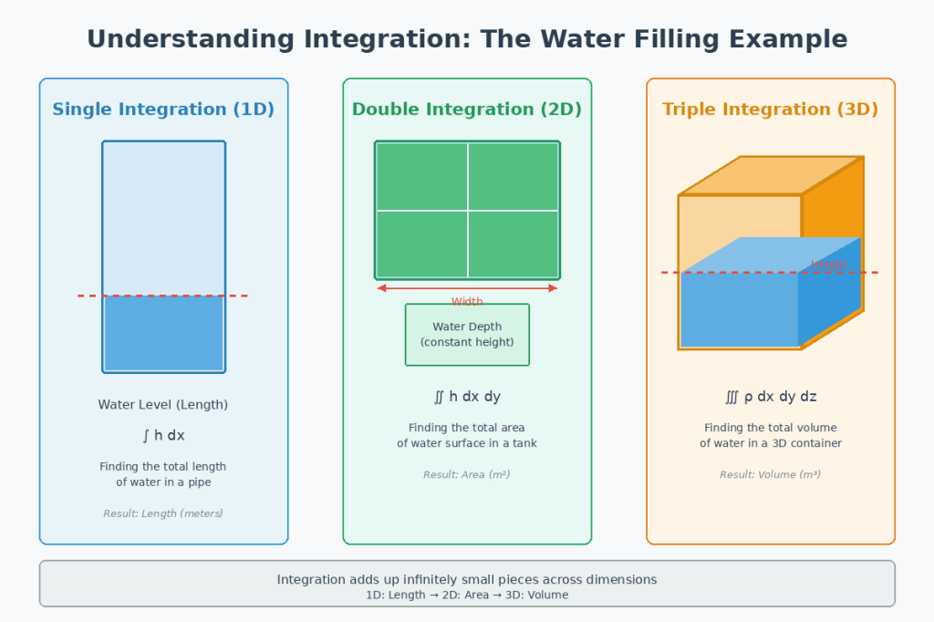
Chapter 2: 📊 From Single to Triple Integration – Adding Dimensions!
Integration comes in different flavors depending on what we’re measuring. Let’s explore them using real-world examples! 🌍
2.1 Single Integration – The Line 📏
What it measures: Length, total accumulation along a path, or area under a curve
Symbol: ∫ f(x) dx
Real-Life Example – Mobile Signal Along a Road:
Imagine you’re driving from your home to work, and you want to know the total mobile signal strength you experienced along the entire route. 📱
At each point on the road, your phone measures signal strength S(x) where x is your position. To find the total signal accumulation, you integrate:
Total Signal = ∫ S(x) dx
This single integration adds up signal strength along a one-dimensional path. It’s like measuring the length of a rope or calculating the work done pushing a box across the floor! 🎯
2.2 Double Integration – The Surface 🎨
What it measures: Area, volume under a surface, or accumulation across a region
Symbol: ∬ f(x,y) dA or ∫∫ f(x,y) dx dy
Real-Life Example – Mobile Signal Coverage in a City:
Now let’s think bigger! Imagine you want to measure the total signal coverage across an entire city. The city is a two-dimensional surface with x (east-west) and y (north-south) coordinates. 🏙️
At every point (x, y) in the city, there’s a signal strength S(x, y). To find the total signal coverage, you use a double integral:
Total Coverage = ∬ S(x,y) dA
This is like painting a floor—you’re covering a two-dimensional area. Other examples include calculating the total rainfall over a region or finding the mass of a thin plate! 🌧️
2.3 Triple Integration – The Volume 🧊
What it measures: Volume, total mass in 3D space, or accumulation throughout a solid region
Symbol: ∭ f(x,y,z) dV or ∫∫∫ f(x,y,z) dx dy dz
Real-Life Example – 3D Mobile Signal in a Skyscraper:
Let’s go even bigger! Imagine a tall skyscraper 🏢 where signal strength varies not just across floors (x, y) but also with height (z). Maybe the signal is stronger on lower floors and weaker near the top.
At every point (x, y, z) in the building, there’s a signal strength S(x, y, z). To find the total signal throughout the entire building volume, you use a triple integral:
Total Signal = ∭ S(x,y,z) dV
This is like filling a swimming pool—you’re filling a three-dimensional space. Other examples include calculating the mass of a solid object or the total heat in a room! 🏊
2.4 Comparing Line, Surface, and Volume 🎯
Let’s connect these to familiar geometric concepts:
- Single Integration (Line Integral): Think of walking along a path and measuring something continuously. Like measuring fence length or cable length along a curved path. 📐
- Double Integration (Surface Integral): Think of covering an area with paint or carpet. You’re measuring across a flat or curved surface. Like calculating how much paint you need for a wall. 🎨
- Triple Integration (Volume Integral): Think of filling a container with water or sand. You’re measuring throughout a three-dimensional space. Like calculating how much water fills a swimming pool. 💧
Chapter 2 in Detail :
Chapter 2: 📊 From Single to Triple Integration – Adding Dimensions!
Integration comes in different flavors depending on what we’re measuring. Let’s explore them using real-world examples, starting from the ground up! 🌍
2.1 Single Integration – The Line 📏
What it measures
Length, total accumulation along a path, or area under a curve
Symbol
∫ f(x) dx
The Building Block Concept 🧱
Think of single integration as stacking tiny slices side by side along a straight line or curve. Imagine you have a very long sandwich, and you want to know its total length. You could measure it inch by inch, then add up all those tiny measurements. That’s exactly what single integration does—but with infinitely thin slices!
Visual Analogy – The Staircase 🪜
Picture climbing a staircase where each step has a different height. If you want to know the total vertical distance you climbed, you’d add up the height of each individual step:
Total height = height₁ + height₂ + height₃ + … + heightₙ
Single integration does this with infinitely many infinitely thin steps, giving you a smooth, precise answer.
Real-Life Example 1: Mobile Signal Along a Road 📱
Imagine you’re driving from your home to work (let’s say 20 kilometers), and you want to know the total mobile signal strength you experienced along the entire route.
At each point on the road, your phone measures signal strength S(x), where x is your position (in kilometers from home). The signal might be:
- Strong (5 bars) near cell towers
- Weak (1 bar) in tunnels or remote areas
- Moderate (3 bars) everywhere else
To find the total signal accumulation:
Total Signal = ∫₀²⁰ S(x) dx
This single integration adds up signal strength along a one-dimensional path.
Concrete Example:
- From km 0-5: S(x) = 4 bars (near city)
- From km 5-15: S(x) = 2 bars (highway, spotty coverage)
- From km 15-20: S(x) = 5 bars (near work, cell tower)
The integral calculates: (4×5) + (2×10) + (5×5) = 20 + 20 + 25 = 65 bar-kilometers
Real-Life Example 2: Work Done Pushing a Box 📦
Imagine pushing a heavy box across a 10-meter room. The friction force varies:
- First 3 meters: 50 Newtons (carpet is thick)
- Next 4 meters: 30 Newtons (wooden floor)
- Last 3 meters: 40 Newtons (slight uphill slope)
Work = ∫ Force(x) dx = (50×3) + (30×4) + (40×3) = 390 Joules
Real-Life Example 3: Water Flow in a River 🌊
A river flows at different speeds along its course. To find the total volume of water that passes a checkpoint in one hour:
Volume = ∫ flow_rate(time) dt
If the flow is:
- 100 liters/min for the first 20 minutes
- 150 liters/min for the next 30 minutes
- 80 liters/min for the last 10 minutes
Total = (100×20) + (150×30) + (80×10) = 7,300 liters
Key Takeaway 🔑
Single integration is about adding up contributions along a one-dimensional path—whether that’s distance, time, or any other single variable. It’s like measuring a rope, calculating calories burned during a jog, or finding the total cost of a taxi ride where the fare changes per kilometer!
2.2 Double Integration – The Surface 🎨
What it measures
Area, volume under a surface, or accumulation across a region
Symbol
∫∫ f(x,y) dA or ∫∫ f(x,y) dx dy
The Building Block Concept 🧱
Double integration is like laying down tiles on a floor. First, you lay tiles in a row (that’s the inner integral), then you add row after row (that’s the outer integral) until the entire floor is covered.
Another way to think about it: If single integration stacks slices in a line, double integration stacks these lines side by side to cover an entire area!
Visual Analogy – Painting a Wall 🖌️
Imagine painting a rectangular wall that’s 4 meters wide and 3 meters tall:
- First pass (inner integral): You paint a vertical stripe from top to bottom (covering 3 meters of height)
- Second pass (outer integral): You repeat this stripe painting, moving left to right across the 4-meter width
Total area painted = ∫∫ dA = 4 × 3 = 12 square meters
Real-Life Example 1: Mobile Signal Coverage in a City 🏙️
Now let’s think bigger! Imagine you want to measure the total signal coverage across an entire city. The city is a two-dimensional surface with:
- x-axis: East-West direction (say, 10 km)
- y-axis: North-South direction (say, 8 km)
At every point (x, y) in the city, there’s a signal strength S(x, y). Maybe:
- Downtown (center): 5 bars
- Suburbs (edges): 3 bars
- Parks (no towers nearby): 1 bar
To find the total signal coverage:
Total Coverage = ∫∫ S(x,y) dA
How it works:
- Pick a north-south line (fix x at some value, say x = 2 km)
- Integrate signal strength along that line from y = 0 to y = 8 km
- Now slide that line from x = 0 to x = 10 km, integrating all those vertical strips
It’s like mowing a lawn in parallel strips! 🏡
Concrete Example: If the city is divided into zones:
- Zone 1 (downtown, 2×2 km): average 5 bars → contributes 5×4 = 20
- Zone 2 (residential, 6×6 km): average 3 bars → contributes 3×36 = 108
- Zone 3 (outskirts, remaining area): average 2 bars → contributes 2×(80-40) = 80
Total ≈ 208 bar-square-kilometers
Real-Life Example 2: Rainfall Over a Region 🌧️
A storm passes over a rectangular farm (5 km × 3 km). Rainfall varies across the farm:
- Northern section: 10 mm
- Central section: 15 mm
- Southern section: 5 mm
Total rainfall volume = ∫∫ rainfall(x,y) dA
If each section is 5 km × 1 km: = (10×5×1) + (15×5×1) + (5×5×1) = 50 + 75 + 25 = 150 cubic kilometers of water
Real-Life Example 3: Solar Panel Energy Collection ☀️
A solar farm has panels spread across a 100m × 50m field. Sunlight intensity varies:
- Center (no shade): 1000 W/m²
- Edges (partial shade from trees): 600 W/m²
Total power = ∫∫ intensity(x,y) dA
This tells you how much total energy the entire solar farm collects!
Innovative Analogy – The Spreadsheet Model 📊
Think of a double integral like summing all cells in an Excel spreadsheet:
     Column1  Column2  Column3  Column4
Row1    5        3        4        2
Row2    6        5        3        4
Row3    4        2        5        3
- Inner integral: Sum down each column (that’s integrating over y)
- Outer integral: Add up all column totals (that’s integrating over x)
Total = (5+6+4) + (3+5+2) + (4+3+5) + (2+4+3) = 15+10+12+9 = 46
Key Takeaway 🔑
Double integration is about adding up contributions across a two-dimensional area—whether that’s a field, a city, a lake, or any flat/curved surface. It’s like calculating the total weight of snow on a roof, the amount of fertilizer needed for a farm, or the total heat absorbed by a solar panel field!
2.3 Triple Integration – The Volume 🧊
What it measures
Volume, total mass in 3D space, or accumulation throughout a solid region
Symbol
∫∫∫ f(x,y,z) dV or ∫∫∫ f(x,y,z) dx dy dz
The Building Block Concept 🧱
Triple integration is like stacking sheets of paper to form a 3D book:
- Single integration: Draw a line on one sheet (1D)
- Double integration: Fill an entire sheet with writing (2D)
- Triple integration: Stack hundreds of sheets to create a thick book (3D)
Alternatively, think of it as filling a swimming pool layer by layer, where each layer is a double integral!
Visual Analogy – Building a Skyscraper 🏗️
Imagine constructing a building:
- First step (inner integral): Build one vertical column from ground to top (integrate over z, height)
- Second step (middle integral): Repeat columns in a row from left to right (integrate over x, width)
- Third step (outer integral): Add row after row from front to back (integrate over y, depth)
You’ve now filled the entire 3D volume of the building!
Real-Life Example 1: 3D Mobile Signal in a Skyscraper 🏢
Let’s go even bigger! Imagine a tall skyscraper:
- x-axis: West to East (50 meters)
- y-axis: South to North (30 meters)
- z-axis: Ground to roof (200 meters, 50 floors)
Signal strength S(x, y, z) varies throughout:
- Lower floors (z = 0-50m): 5 bars (street-level cell towers)
- Middle floors (z = 50-150m): 4 bars (good coverage)
- Upper floors (z = 150-200m): 2 bars (far from towers)
To find the total signal throughout the entire building:
Total Signal = ∫∫∫ S(x,y,z) dV
How it works:
- Pick a vertical column at position (x=10m, y=15m)
- Integrate signal from ground to roof (z: 0→200m)
- Slide this column across the floor in the x-direction (x: 0→50m)
- Repeat for all rows in the y-direction (y: 0→30m)
Concrete Calculation: Volume of building = 50 × 30 × 200 = 300,000 m³
If average signal = (5×1/4) + (4×1/2) + (2×1/4) = 1.25 + 2 + 0.5 = 3.75 bars
Total ≈ 3.75 × 300,000 = 1,125,000 bar-cubic-meters
Real-Life Example 2: Temperature in a Room 🌡️
A room (4m × 5m × 3m high) has varying temperature:
- Near the heater (bottom corner): 25°C
- Center of room: 20°C
- Near the ceiling: 18°C (heat rises, but not all the way to ceiling)
Total thermal energy = ∫∫∫ temperature(x,y,z) × air_density × specific_heat dV
This tells you how much total heat energy is stored in the air filling that room!
Real-Life Example 3: Mass of a Sculpture 🗿
An artist creates a concrete sculpture (2m × 1m × 1.5m). The density varies:
- Base (thick concrete): 2400 kg/m³
- Middle: 2000 kg/m³
- Top (hollow sections): 1200 kg/m³
Total mass = ∫∫∫ density(x,y,z) dV
Without calculus: You’d have to weigh the entire sculpture. With triple integration: You can calculate the mass by summing up tiny density contributions throughout the volume!
Real-Life Example 4: Pollution in the Atmosphere 🏭
Imagine measuring smog concentration over a city:
- x, y: City area (10 km × 10 km)
- z: Altitude (0 to 2 km up)
Pollution concentration C(x,y,z) varies:
- Ground level (z=0): 80 µg/m³
- Mid-altitude (z=1km): 40 µg/m³
- Upper altitude (z=2km): 10 µg/m³
Total pollution = ∫∫∫ C(x,y,z) dV
This helps environmental scientists understand total pollutant load in the air!
Innovative Analogy – The Rubik’s Cube Model 🎲
Imagine a Rubik’s Cube where each small cube has a number inside it:
Layer 1 (bottom):[5][3][4][2][6][3][4][5][2]Layer 2 (middle):[3][4][5][6][2][4][3][5][3]Layer 3 (top):[2][3][4][4][5][3][3][4][2]
- First integration: Sum across each row (integrate over x)
- Second integration: Sum all rows in a layer (integrate over y)
- Third integration: Stack and sum all layers (integrate over z)
Total = Sum of all 27 little cubes!
Innovative Analogy – The Aquarium Model 🐠
Think of filling an aquarium with water:
- Pour water into a thin vertical tube (single integral, line)
- Expand that tube into a thin vertical sheet (double integral, surface)
- Thicken that sheet to fill the entire tank (triple integral, volume)
Each step adds a dimension!
2.4 Comparing Line, Surface, and Volume 🎯
Let’s connect these to familiar geometric concepts with a unifying story:
The Pizza Delivery Story 🍕
Single Integration (Line): You deliver pizza along a street. You measure the total distance traveled and fuel consumed along that one-dimensional route.
- What you’re measuring: Length along a path
- Analogy: Measuring fence length, cable length, or a hiking trail
- Dimension: 1D (just position along the path)
Double Integration (Surface): Now you deliver to an entire neighborhood. You measure total area covered and number of houses served across a two-dimensional region.
- What you’re measuring: Area across a surface
- Analogy: Painting a wall, carpeting a floor, mowing a lawn
- Dimension: 2D (position has two coordinates: x and y)
Triple Integration (Volume): Now you’re delivering to a massive apartment complex (like a skyscraper). You measure total volume of the building and number of apartments throughout the three-dimensional space.
- What you’re measuring: Volume throughout a solid
- Analogy: Filling a pool, air-conditioning a building, measuring mass of an object
- Dimension: 3D (position has three coordinates: x, y, and z)
Quick Reference Table 📋
| Type | Dimensions | Symbol | Measures | Real Example |
|---|---|---|---|---|
| Single | 1D (line) | ∫ f(x) dx | Length, accumulation along path | Signal strength on a road trip |
| Double | 2D (surface) | ∫∫ f(x,y) dA | Area, accumulation over region | Rainfall over a farm |
| Triple | 3D (volume) | ∫∫∫ f(x,y,z) dV | Volume, accumulation in 3D space | Temperature throughout a room |
The Progressive Dimension Song 🎵
To remember the progression:
- 1D: “Walk the line, add up fine!” (walking along a path)
- 2D: “Paint the floor, wall to wall!” (covering an area)
- 3D: “Fill it up, to the top!” (filling a volume)
Key Insight 💡
Each type of integration adds one more dimension:
- Start with a point (0D)
- Integrate once → get a line (1D)
- Integrate twice → get a surface (2D)
- Integrate three times → get a volume (3D)
It’s like going from a dot → to a stroke → to a painting → to a sculpture!
Chapter 3: 📚 The Essential Rules of Single Integration
Chapter 3: 🎯 Integration Rules – Your Mathematical Superpowers!
Now that you understand what integration is, let’s learn how to do it! Here are the fundamental rules you’ll use over and over again. Don’t worry—we’ll make them simple! 💪
Think of these rules as shortcuts or cheat codes 🎮 that make solving integrals way easier than doing everything from scratch!
3.1 The Symbol ∫ – Your New Best Friend 🤝
Meet the Integral Sign! 👋
The symbol ∫ is called an integral sign. It’s like a fancy, stretched-out letter ‘S’ (which stands for ‘Sum’) because integration is really about summing up infinitely many tiny pieces!
Think of it as a magic wand ✨ that says: “Let’s add up ALL the little bits!”
How to Read Integration Notation 📖
When you see: ∫ f(x) dx
Read it as: “the integral of f(x) with respect to x”
Let’s break down what each part means:
| Symbol | Name | What It Means | Analogy |
|---|---|---|---|
| ∫ | Integral sign | “Let’s integrate!” or “Let’s sum up!” | The action command, like pressing “GO!” 🚦 |
| f(x) | The function | What we’re adding up | The ingredient we’re measuring 🥄 |
| dx | Differential | “With respect to x” (our variable of summation) | The tiny slice thickness 🍰 |
Visual Breakdown 🎨
     ∫  x²  dx
     ↑  ↑   ↑
     │  │   │
     │  │   └── "Cut into tiny pieces in the x-direction"
     │  └────── "The thing we're integrating" (the height)
     └───────── "Add them all up!"
Real-Life Translation:
Imagine you’re slicing a loaf of bread 🍞:
- ∫ = “Add up all the slices”
- x² = “Each slice has a certain thickness based on x²”
- dx = “Each slice is infinitely thin in the x-direction”
The result tells you the total volume of bread when you add up all those super-thin slices!
Another Way to Think About It 🧠
∫ f(x) dx is like saying:
“Hey! Take this function f(x), chop it into infinitely many tiny pieces of width dx, and add them all up!”
It’s like:
- 🧮 Adding up all the grains of sand on a beach to get the total volume
- 💧 Adding up all the tiny droplets in a river to measure total water flow
- 📊 Adding up sales from every single minute of the day to get total revenue
The “dx” – Why Is It There? 🤔
The dx is super important! It tells you:
- Which variable you’re integrating with respect to (in this case, x)
- How thin each slice is (infinitely thin!)
- The direction you’re slicing (along the x-axis)
Example:
- ∫ f(x) dx → integrate along the x-direction (horizontal slices 📏)
- ∫ f(y) dy → integrate along the y-direction (vertical slices 📐)
- ∫ f(t) dt → integrate over time (time slices ⏰)
Quick Memory Trick 🧠✨
∫ looks like a stretched S → S for Sum → Integration Sums things up!
3.2 The Golden Rules of Integration ⚡
Think of these rules as your mathematical superpowers 🦸! They make integration WAY easier by breaking down complex problems into simple pieces.
🔢 Rule 1: Constant Multiple Rule – “Pull Out the Number!”
The Rule:
∫ k·f(x) dx = k·∫ f(x) dx
Translation in Simple English 🗣️:
“If you have a number (constant) multiplied by your function, you can pull that number OUT of the integral and deal with it later!”
It’s like having a coupon that says “Buy 5 of these!” You don’t need to apply the “×5” to every single step—just multiply your answer by 5 at the end! 🛒
Visual Example 🎨:
Problem: ∫ 5x² dx
What the rule says: “See that 5? It’s just a constant multiplier. Pull it out front!”
∫ 5x² dx = 5 · ∫ x² dx
Now you only need to integrate x², and then multiply the result by 5 at the end!
Real-Life Analogy 🍕:
Imagine you’re calculating the total cost of 5 pizzas, where each pizza costs $x² (maybe the price changes based on size x).
Option 1 (hard way): Calculate the cost of each of the 5 pizzas separately and add them up.
Option 2 (smart way): Calculate the cost of ONE pizza, then multiply by 5!
That’s exactly what the Constant Multiple Rule does! 🎯
More Examples:
| Problem | Apply Rule | Simplified |
|---|---|---|
| ∫ 7x³ dx | 7 · ∫ x³ dx | Pull out the 7 |
| ∫ -3sin(x) dx | -3 · ∫ sin(x) dx | Pull out the -3 |
| ∫ 10e^x dx | 10 · ∫ e^x dx | Pull out the 10 |
| ∫ (1/2)x dx | (1/2) · ∫ x dx | Pull out the 1/2 |
Why This Rule Rocks 🎸:
✅ Makes integrals simpler to solve
✅ Saves time and reduces mistakes
✅ Works with ANY constant (positive, negative, fractions, decimals!)
Key Insight: Constants are like passengers 🚗 in a car. They just sit there and don’t affect the driving (integration). So let them sit outside the integral!
➕ Rule 2: Sum Rule – “Break It Into Pieces!”
The Rule:
∫ [f(x) + g(x)] dx = ∫ f(x) dx + ∫ g(x) dx
Translation in Simple English 🗣️:
“If you’re integrating a SUM of functions, you can integrate each function separately and then add the results!”
It’s like cleaning your room 🧹: Instead of trying to clean everything at once, you clean your desk first, then your bed, then your floor, and combine the efforts!
Visual Example 🎨:
Problem: ∫ (x² + 3x) dx
What the rule says: “You have TWO things being added: x² and 3x. Integrate them separately!”
∫ (x² + 3x) dx = ∫ x² dx + ∫ 3x dx
Now tackle each piece one at a time! Much easier! 😊
Real-Life Analogy 🍔🍟:
Imagine calculating the total calories you ate today. You had:
- A burger 🍔 (calories = B)
- Fries 🍟 (calories = F)
Total calories = Calories from burger + Calories from fries = B + F
You don’t need to analyze them together—just calculate each separately and add them up!
More Examples:
| Problem | Apply Rule | Simplified |
|---|---|---|
| ∫ (x³ + 5x²) dx | ∫ x³ dx + ∫ 5x² dx | Split into two integrals |
| ∫ (sin(x) + cos(x)) dx | ∫ sin(x) dx + ∫ cos(x) dx | Split into two integrals |
| ∫ (2x + 7) dx | ∫ 2x dx + ∫ 7 dx | Split into two integrals |
| ∫ (e^x + x²) dx | ∫ e^x dx + ∫ x² dx | Split into two integrals |
Combo Power! 💥 Combining Rule 1 and Rule 2:
Let’s use BOTH rules together!
Problem: ∫ (4x² + 6x) dx
Step 1: Use Sum Rule (split it up) = ∫ 4x² dx + ∫ 6x dx
Step 2: Use Constant Multiple Rule (pull out constants) = 4·∫ x² dx + 6·∫ x dx
Now you just need to integrate x² and x separately! 🎉
Why This Rule Rocks 🎸:
✅ Breaks complicated integrals into simple pieces
✅ You can tackle one term at a time (less overwhelming!)
✅ Works with ANY number of terms (3, 4, 10, 100 terms!)
Key Insight: Integration is linear, which means it plays nicely with addition. You can split and conquer! 🗡️
➖ Rule 3: Difference Rule – “Subtraction Works Too!”
The Rule:
∫ [f(x) – g(x)] dx = ∫ f(x) dx – ∫ g(x) dx
Translation in Simple English 🗣️:
“Just like the Sum Rule, but with subtraction! Integrate each part separately, then subtract!”
It’s the same idea as Rule 2, just with a minus sign instead of a plus! 🎯
Visual Example 🎨:
Problem: ∫ (x³ – 2x) dx
What the rule says: “You’re subtracting two things: x³ and 2x. Integrate them separately!”
∫ (x³ – 2x) dx = ∫ x³ dx – ∫ 2x dx
Easy peasy! 🍋
Real-Life Analogy 💰:
Imagine calculating your net savings this month:
- You earned $E 💵
- You spent $S 💸
Net savings = Earned – Spent = E – S
You calculate each separately, then subtract! Same with integration!
More Examples:
| Problem | Apply Rule | Simplified |
|---|---|---|
| ∫ (5x² – 3x) dx | ∫ 5x² dx – ∫ 3x dx | Split into two integrals |
| ∫ (cos(x) – sin(x)) dx | ∫ cos(x) dx – ∫ sin(x) dx | Split into two integrals |
| ∫ (e^x – x) dx | ∫ e^x dx – ∫ x dx | Split into two integrals |
| ∫ (10 – x²) dx | ∫ 10 dx – ∫ x² dx | Split into two integrals |
All Three Rules Together! 🎪
Let’s combine ALL THREE RULES in one mega-example!
Problem: ∫ (6x³ – 4x² + 2x) dx
Step 1: Use Sum/Difference Rule (split into pieces) = ∫ 6x³ dx – ∫ 4x² dx + ∫ 2x dx
Step 2: Use Constant Multiple Rule (pull out constants) = 6·∫ x³ dx – 4·∫ x² dx + 2·∫ x dx
Now you just integrate the simple parts: x³, x², and x! 🎉
Why This Rule Rocks 🎸:
✅ Same power as the Sum Rule, just with subtraction
✅ Makes complex expressions manageable
✅ Combines perfectly with the other rules
Key Insight: Addition and subtraction both work the same way in integration. Split, integrate, then combine! 🧩
🎯 Quick Summary Table – The Big Three Rules
| Rule | Formula | What It Does | Memory Trick |
|---|---|---|---|
| Constant Multiple 🔢 | ∫ k·f(x) dx = k·∫ f(x) dx | Pull constants outside | Constants are passengers 🚗 |
| Sum Rule ➕ | ∫ [f + g] dx = ∫ f dx + ∫ g dx | Split addition into pieces | Clean room piece by piece 🧹 |
| Difference Rule ➖ | ∫ [f – g] dx = ∫ f dx – ∫ g dx | Split subtraction into pieces | Earnings minus spending 💰 |
🧠 Memory Tricks & Tips
🎵 The Integration Song:
“Pull out constants, split the sums,
Integration’s easy when you know what comes!
Add or subtract, it’s all the same,
Break it apart and win the game!” 🎶
🎨 Visual Reminder:
Think of integration like eating a multi-layer cake 🎂:
- Constant Multiple Rule: If you have 3 cakes, eat one and multiply by 3!
- Sum Rule: Layer 1 + Layer 2 + Layer 3 = Eat each layer separately
- Difference Rule: Whole cake – Eaten slice = Calculate separately then subtract
🎮 The Video Game Analogy:
Integration rules are like combo moves in a fighting game:
- Rule 1: Boost move (multiply damage)
- Rule 2: Chain attack (link multiple hits)
- Rule 3: Counter move (subtract opponent’s defense)
Use them together for maximum power! 💥
⚠️ Common Mistakes to Avoid!
❌ Mistake 1: Forgetting the “dx”
Wrong: ∫ 5x²
Right: ∫ 5x² dx ✅
Always include the dx! It tells you what variable you’re integrating!
❌ Mistake 2: Trying to pull non-constants out
Wrong: ∫ x·sin(x) dx = x·∫ sin(x) dx ❌
Right: Keep x inside (it’s NOT a constant!)
Only pull out numbers that don’t depend on x!
❌ Mistake 3: Splitting multiplication (NOT addition)
Wrong: ∫ x·cos(x) dx = ∫ x dx · ∫ cos(x) dx ❌
Right: Use a different technique (integration by parts – coming later!)
The Sum/Difference rules ONLY work for addition/subtraction, NOT multiplication!
🚀 Practice Challenge!
Try simplifying these using the three golden rules:
- ∫ (8x⁴ + 3x²) dx
- ∫ (10sin(x) – 5cos(x)) dx
- ∫ (2e^x + 7x – 3) dx
Hint: Use all three rules! Pull out constants, then split the terms! 💪
Next up: We’ll learn the Power Rule – the most commonly used integration formula that makes solving x², x³, x⁴ (and more!) super easy! 🎯✨
Chapter 3.3: 🚀 The Power Rule – Your Most Powerful Tool!
The Power Rule is THE most important integration formula you’ll ever learn! It works for x², x³, x⁴, and basically any power of x. Master this, and you’ll solve 80% of basic integrals! 💪✨
🎯 The Power Rule Formula
The Magic Formula:
∫ xⁿ dx = (xⁿ⁺¹)/(n+1) + C
where n ≠ -1
In Plain English 🗣️:
“To integrate x to any power, add 1 to the exponent, then divide by that new exponent. Don’t forget to add C at the end!”
🤔 Breaking Down the Formula
Let’s understand each piece:
∫ xⁿ dx = xⁿ⁺¹/(n+1) + C ↑ ↑ ↑ ↑ ↑ │ │ │ │ │ │ │ │ │ └── Constant of integration (ALWAYS needed!) │ │ │ └───────── Divide by the NEW exponent │ │ └─────────────── Add 1 to the exponent │ └───────────────────── The power we're integrating └──────────────────────── Integrate this!
🎨 Step-by-Step Process
The 3-Step Power Rule Dance 💃:
Step 1: 👆 Add 1 to the exponent
Step 2: ➗ Divide by the new exponent
Step 3: ➕ Add C (the constant of integration)
📚 Simple Examples – Let’s See It in Action!
Example 1: Integrating x²
Problem: ∫ x² dx
Step 1: The exponent is 2. Add 1 → 2 + 1 = 3
Step 2: Divide by the new exponent (3) = x³/3
Step 3: Add C = x³/3 + C ✅
Visual Check:
- Started with: x² (exponent = 2)
- Ended with: x³/3 (exponent = 3, divided by 3) ✅
Example 2: Integrating x⁵
Problem: ∫ x⁵ dx
Step 1: Exponent is 5. Add 1 → 5 + 1 = 6
Step 2: Divide by 6 = x⁶/6
Step 3: Add C = x⁶/6 + C ✅
Example 3: Integrating x (which is really x¹)
Problem: ∫ x dx
Remember: x = x¹ (the exponent is 1)
Step 1: Add 1 → 1 + 1 = 2
Step 2: Divide by 2 = x²/2
Step 3: Add C = x²/2 + C ✅
Example 4: Integrating just 1 (which is x⁰)
Problem: ∫ 1 dx
Remember: 1 = x⁰ (anything to the power 0 equals 1)
Step 1: Add 1 → 0 + 1 = 1
Step 2: Divide by 1 = x¹/1 = x
Step 3: Add C = x + C ✅
Real-Life Meaning: Integrating 1 gives you x! Makes sense—if you add up 1 + 1 + 1… many times, you get a total!
🎪 More Examples – Getting Fancy!
Example 5: Integrating x⁷
∫ x⁷ dx = x⁸/8 + C
👉 Exponent 7 → add 1 → becomes 8 → divide by 8 ✅
Example 6: Integrating x¹⁰
∫ x¹⁰ dx = x¹¹/11 + C
👉 Exponent 10 → add 1 → becomes 11 → divide by 11 ✅
Example 7: Integrating x⁰·⁵ (Square Root!)
Problem: ∫ √x dx
First, rewrite the square root: √x = x^(1/2)
Step 1: Add 1 to 1/2 → 1/2 + 1 = 3/2
Step 2: Divide by 3/2 (which means multiply by 2/3) = x^(3/2) · (2/3) = (2/3)x^(3/2)
Step 3: Add C = (2/3)x^(3/2) + C ✅
Or you can write it as: (2/3)√(x³) + C 🎯
🔥 Working with Negative Exponents!
The Power Rule works with negative exponents too!
Example 8: Integrating 1/x²
Problem: ∫ (1/x²) dx
Step 1: Rewrite using negative exponents: 1/x² = x⁻²
Step 2: Apply Power Rule:
- Add 1 to -2 → -2 + 1 = -1
- Divide by -1
= x⁻¹/(-1) = -x⁻¹ = -1/x
Step 3: Add C = -1/x + C ✅
Example 9: Integrating 1/x³
∫ (1/x³) dx
Rewrite: 1/x³ = x⁻³
Apply Power Rule:
- Exponent -3 → add 1 → -2
- Divide by -2
= x⁻²/(-2) = -1/(2x²) + C ✅
Example 10: Integrating 1/√x
∫ (1/√x) dx
Rewrite: 1/√x = x⁻¹/²
Apply Power Rule:
- Exponent -1/2 → add 1 → 1/2
- Divide by 1/2 (multiply by 2)
= 2x^(1/2) = 2√x + C ✅
🎨 Visual Pattern Recognition
Notice the beautiful pattern! 👀
| Integrating | Result | Pattern |
|---|---|---|
| ∫ x⁰ dx | x + C | 0→1 |
| ∫ x¹ dx | x²/2 + C | 1→2, ÷2 |
| ∫ x² dx | x³/3 + C | 2→3, ÷3 |
| ∫ x³ dx | x⁴/4 + C | 3→4, ÷4 |
| ∫ x⁴ dx | x⁵/5 + C | 4→5, ÷5 |
| ∫ x⁵ dx | x⁶/6 + C | 5→6, ÷6 |
The Pattern: Exponent n becomes (n+1) and we divide by (n+1)! 🎯
🌟 What About That Mysterious “+C”?
Why Do We Add C? 🤔
The +C is called the constant of integration, and it’s SUPER important!
The Reason:
When you differentiate (reverse of integration), constants disappear!
For example:
- d/dx (x² + 5) = 2x
- d/dx (x² + 100) = 2x
- d/dx (x² – 37) = 2x
All three give the same derivative (2x), even though they’re different functions!
So when we integrate backwards: ∫ 2x dx = x² + C
The C represents any possible constant that could have been there! It could be 5, 100, -37, or ANY number! 🎲
Real-Life Analogy 🚗:
Imagine you’re told: “You drove at 60 mph for 2 hours.”
You can calculate the distance traveled (120 miles), but you don’t know your starting position!
- Did you start at mile marker 0? (position = 120)
- Did you start at mile marker 50? (position = 170)
- Did you start at mile marker 200? (position = 320)
The C represents that unknown starting point! 🏁
Important Rules About C:
✅ ALWAYS include +C in indefinite integrals
✅ C represents any constant (could be 0, 1, -5, 1000, π, etc.)
✅ Different problems might have different C values
✅ Only drop C when solving definite integrals (limits of integration)
🎪 Combining Power Rule with Our Golden Rules!
Let’s use ALL our rules together! 💥
Example 11: Multi-Term Integration
Problem: ∫ (3x⁴ + 5x² – 2x) dx
Step 1: Split using Sum/Difference Rule ➕➖ = ∫ 3x⁴ dx + ∫ 5x² dx – ∫ 2x dx
Step 2: Pull out constants using Constant Multiple Rule 🔢 = 3∫ x⁴ dx + 5∫ x² dx – 2∫ x dx
Step 3: Apply Power Rule to each term 🚀
- ∫ x⁴ dx = x⁵/5
- ∫ x² dx = x³/3
- ∫ x dx = x²/2
Step 4: Multiply by constants and combine = 3(x⁵/5) + 5(x³/3) – 2(x²/2)
= (3x⁵)/5 + (5x³)/3 – x² + C ✅
Example 12: Mix of Everything!
Problem: ∫ (6x³ – 4√x + 2/x²) dx
Step 1: Rewrite in exponent form = ∫ (6x³ – 4x^(1/2) + 2x⁻²) dx
Step 2: Split and pull out constants = 6∫ x³ dx – 4∫ x^(1/2) dx + 2∫ x⁻² dx
Step 3: Apply Power Rule to each
- ∫ x³ dx = x⁴/4
- ∫ x^(1/2) dx = x^(3/2)/(3/2) = (2/3)x^(3/2)
- ∫ x⁻² dx = x⁻¹/(-1) = -1/x
Step 4: Combine = 6(x⁴/4) – 4(2/3)x^(3/2) + 2(-1/x) + C
= (3x⁴)/2 – (8x^(3/2))/3 – 2/x + C ✅
🚫 The ONE Exception – When n = -1
What Happens with 1/x?
Problem: ∫ (1/x) dx = ∫ x⁻¹ dx
If we tried Power Rule:
- Add 1 to -1 → get 0
- Divide by 0 → UNDEFINED! 💥
The Power Rule DOESN’T work when n = -1!
Special Case Answer:
∫ (1/x) dx = ln|x| + C 📊
(We use the natural logarithm instead!)
Memory Trick: 1/x is the rebel 😎 – it doesn’t follow the Power Rule! It gets its own special answer: ln|x|!
🎯 Quick Reference Table
| Integral | Answer | Notes |
|---|---|---|
| ∫ x⁰ dx | x + C | Just 1 integrated |
| ∫ x dx | x²/2 + C | Linear function |
| ∫ x² dx | x³/3 + C | Parabola |
| ∫ x³ dx | x⁴/4 + C | Cubic |
| ∫ xⁿ dx | x^(n+1)/(n+1) + C | General Power Rule (n ≠ -1) |
| ∫ √x dx | (2/3)x^(3/2) + C | Rewrite as x^(1/2) first |
| ∫ 1/x² dx | -1/x + C | Rewrite as x⁻² first |
| ∫ 1/x dx | ln | x |
🧠 Memory Tricks & Mnemonics
🎵 The Power Rule Song:
“Add one to the power, that’s what you do,
Then divide by the new one, it’s easy for you!
Don’t forget C at the end of the line,
Power Rule integration works every time!” 🎶
🎨 Visual Memory Aid:
Think of stairs going UP 🪜:
- Start at step n
- Go UP one step to n+1 👆
- Then divide by that new step number ➗
- Add your C for completion ✅
🎮 Video Game Analogy:
Power Rule is like leveling up in a game:
- Your power is xⁿ
- Integration levels you up: xⁿ → xⁿ⁺¹
- But leveling costs points, so divide by (n+1)
- C is your starting XP (unknown until you know initial conditions)
⚠️ Common Mistakes to Avoid!
❌ Mistake 1: Forgetting to add 1
Wrong: ∫ x³ dx = x³/3 + C
Right: ∫ x³ dx = x⁴/4 + C ✅
Remember: ADD 1 to the exponent FIRST!
❌ Mistake 2: Forgetting the +C
Wrong: ∫ x² dx = x³/3
Right: ∫ x² dx = x³/3 + C ✅
The +C is NOT optional!
❌ Mistake 3: Using Power Rule on 1/x
Wrong: ∫ (1/x) dx = x⁰/0 (undefined!)
Right: ∫ (1/x) dx = ln|x| + C ✅
1/x is the exception!
❌ Mistake 4: Forgetting to rewrite roots and fractions
Wrong: ∫ √x dx = ??? (confused!)
Right: Rewrite as ∫ x^(1/2) dx = (2/3)x^(3/2) + C ✅
Always rewrite in exponent form first!
🏋️ Practice Problems – Build Your Skills!
Try these! (Answers at the bottom)
Level 1 – Beginner 🟢:
- ∫ x⁴ dx
- ∫ x⁶ dx
- ∫ x dx
Level 2 – Intermediate 🟡: 4. ∫ (x² + 3x) dx 5. ∫ (5x³ – 2x²) dx 6. ∫ √x dx
Level 3 – Advanced 🔴: 7. ∫ (4x⁵ – 3/x² + 2) dx 8. ∫ (x³ – 5√x + 1/x³) dx 9. ∫ (2x⁴ – 6x² + 8x – 3) dx
🎊 Answers to Practice Problems:
- x⁵/5 + C
- x⁷/7 + C
- x²/2 + C
- x³/3 + (3x²)/2 + C
- (5x⁴)/4 – (2x³)/3 + C
- (2/3)x^(3/2) + C
- (2x⁶)/3 + 3/x + 2x + C
- x⁴/4 – (10/3)x^(3/2) + 1/(2x²) + C
- (2x⁵)/5 – 2x³ + 4x² – 3x + C
How did you do? 🎯
🚀 Level Up Achievement Unlocked!
Congratulations! 🎉 You’ve mastered the Power Rule—one of the most powerful tools in calculus!
You can now integrate: ✅ Polynomials (x², x³, x⁴…) ✅ Roots (√x, ∛x…) ✅ Fractions (1/x², 1/x³…) ✅ Combined expressions with multiple terms!
Next up: We’ll learn special integration formulas for trigonometric functions (sin, cos, tan), exponentials (eˣ), and more! 🎯✨
Chapter 4: 🎯 Essential Integration Formulas
📚 Complete Integration Guide – WordPress Edition
Welcome to the wonderful world of Integration! 🎉
This comprehensive guide will take you from absolute beginner to integration master, using simple language, real-world examples, and plenty of emojis to keep things fun! 😊
Chapter 1: 🎯 What is Integration? – The Big Picture
1.1 The Simple Idea 💡
Integration is just fancy addition!
Imagine you want to find the total area under a curvy hill. You can’t use simple geometry because it’s not a rectangle or triangle. So what do you do?
You break the area into tiny vertical strips (like slicing bread 🍞), find the area of each thin strip, then add them all up!
That’s integration! It’s adding up infinitely many infinitely small pieces to get a total. ✨
1.2 Real-Life Example – Distance from Speed 🚗
The Problem:
You’re driving a car, and your speed keeps changing. How do you find the total distance you traveled?
The Solution:
If you know your speed at every moment, integration adds up all those tiny distances traveled in each tiny moment of time!
- Speed at each moment = s(t)
- Tiny time interval = dt
- Tiny distance = speed × time = s(t) × dt
- Total distance = ∫ s(t) dt (integrate speed over time!)
Concrete Example:
If you drive at 60 mph for 2 hours:
- Distance = ∫ 60 dt from t=0 to t=2
- Distance = 60 × 2 = 120 miles ✅
1.3 Integration vs Differentiation – Two Sides of the Same Coin 🪙
Differentiation (taking derivatives) and Integration are opposites!
Think of it like this:
| Concept | Differentiation | Integration |
|---|---|---|
| Direction | Breaking down ⬇️ | Building up ⬆️ |
| Finds | Rate of change 📊 | Total accumulation 📈 |
| Example | Speed → Acceleration | Speed → Distance |
| Symbol | d/dx or f'(x) | ∫ dx |
| Like | Taking apart a Lego tower 🧱 | Building a Lego tower 🏗️ |
Example:
- If position = x², then velocity = 2x (differentiation)
- If velocity = 2x, then position = x² + C (integration)
They undo each other! 🔄
1.4 The Two Types of Integration 🎭
Type 1: Indefinite Integral (No limits)
Symbol: ∫ f(x) dx = F(x) + C
What it means: Find the general formula for the antiderivative (reverse of derivative).
The +C is MANDATORY! It represents an unknown constant. 📌
Example:
∫ x² dx = x³/3 + C
Why +C? Because when you differentiate x³/3 + 5, you get x². And when you differentiate x³/3 + 100, you also get x². The constant could be anything! 🎲
Type 2: Definite Integral (With limits)
Symbol: ∫[from a to b] f(x) dx = F(b) – F(a)
What it means: Find the exact numerical value of the total accumulation between x=a and x=b.
No +C needed! The constant cancels out. ✅
Example:
∫[from 0 to 3] x² dx = [x³/3] from 0 to 3 = (27/3) – (0/3) = 9
Real-Life: Total water flow in a river between 9am and 5pm 🌊
1.5 Visual Understanding – Area Under the Curve 📊
Integration finds the area between the curve and the x-axis!
Important Rules:
- Area above the x-axis = positive ➕
- Area below the x-axis = negative ➖
- Total area = positive areas – negative areas
Example:
If a sine wave goes above and below the x-axis, the positive and negative areas might cancel out! 🌊
1.6 Quick Summary – What You Need to Know 🎯
✅ Integration = adding up infinite tiny pieces
✅ It’s the opposite of differentiation
✅ Indefinite integral = general formula + C
✅ Definite integral = specific numerical value
✅ Integration finds area under curves
✅ Real-world uses: distance, volume, work, probability, and more!
Chapter 2: 📊 From Single to Triple Integration – Adding Dimensions!
Integration comes in different flavors depending on what we’re measuring. Let’s explore them using real-world examples! 🌍
2.1 Single Integration – The Line 📏
What it measures:
Length, total accumulation along a path, or area under a curve
Symbol:
∫ f(x) dx
The Building Block Concept 🧱
Think of single integration as stacking tiny slices side by side along a straight line or curve. Imagine you have a very long sandwich, and you want to know its total length. You could measure it inch by inch, then add up all those tiny measurements. That’s exactly what single integration does—but with infinitely thin slices!
Visual Analogy – The Staircase 🪜
Picture climbing a staircase where each step has a different height. If you want to know the total vertical distance you climbed, you’d add up the height of each individual step:
Total height = height₁ + height₂ + height₃ + … + heightₙ
Single integration does this with infinitely many infinitely thin steps, giving you a smooth, precise answer.
Real-Life Example 1: Mobile Signal Along a Road 📱
Imagine you’re driving from your home to work (let’s say 20 kilometers), and you want to know the total mobile signal strength you experienced along the entire route.
At each point on the road, your phone measures signal strength S(x), where x is your position (in kilometers from home). The signal might be:
- Strong (5 bars) near cell towers
- Weak (1 bar) in tunnels or remote areas
- Moderate (3 bars) everywhere else
To find the total signal accumulation:
Total Signal = ∫[from 0 to 20] S(x) dx
This single integration adds up signal strength along a one-dimensional path.
Concrete Example:
- From km 0-5: S(x) = 4 bars (near city)
- From km 5-15: S(x) = 2 bars (highway, spotty coverage)
- From km 15-20: S(x) = 5 bars (near work, cell tower)
The integral calculates: (4×5) + (2×10) + (5×5) = 20 + 20 + 25 = 65 bar-kilometers
Real-Life Example 2: Work Done Pushing a Box 📦
Imagine pushing a heavy box across a 10-meter room. The friction force varies:
- First 3 meters: 50 Newtons (carpet is thick)
- Next 4 meters: 30 Newtons (wooden floor)
- Last 3 meters: 40 Newtons (slight uphill slope)
Work = ∫ Force(x) dx = (50×3) + (30×4) + (40×3) = 390 Joules
Real-Life Example 3: Water Flow in a River 🌊
A river flows at different speeds along its course. To find the total volume of water that passes a checkpoint in one hour:
Volume = ∫ flow_rate(time) dt
If the flow is:
- 100 liters/min for the first 20 minutes
- 150 liters/min for the next 30 minutes
- 80 liters/min for the last 10 minutes
Total = (100×20) + (150×30) + (80×10) = 7,300 liters
Key Takeaway 🔑
Single integration is about adding up contributions along a one-dimensional path—whether that’s distance, time, or any other single variable. It’s like measuring a rope, calculating calories burned during a jog, or finding the total cost of a taxi ride where the fare changes per kilometer! 🎯
2.2 Double Integration – The Surface 🎨
What it measures:
Area, volume under a surface, or accumulation across a region
Symbol:
∫∫ f(x,y) dA or ∫∫ f(x,y) dx dy
The Building Block Concept 🧱
Double integration is like laying down tiles on a floor. First, you lay tiles in a row (that’s the inner integral), then you add row after row (that’s the outer integral) until the entire floor is covered.
Another way to think about it: If single integration stacks slices in a line, double integration stacks these lines side by side to cover an entire area!
Visual Analogy – Painting a Wall 🖌️
Imagine painting a rectangular wall that’s 4 meters wide and 3 meters tall:
- First pass (inner integral): You paint a vertical stripe from top to bottom (covering 3 meters of height)
- Second pass (outer integral): You repeat this stripe painting, moving left to right across the 4-meter width
Total area painted = ∫∫ dA = 4 × 3 = 12 square meters
Real-Life Example 1: Mobile Signal Coverage in a City 🏙️
Now let’s think bigger! Imagine you want to measure the total signal coverage across an entire city. The city is a two-dimensional surface with:
- x-axis: East-West direction (say, 10 km)
- y-axis: North-South direction (say, 8 km)
At every point (x, y) in the city, there’s a signal strength S(x, y). Maybe:
- Downtown (center): 5 bars
- Suburbs (edges): 3 bars
- Parks (no towers nearby): 1 bar
To find the total signal coverage:
Total Coverage = ∫∫ S(x,y) dA
How it works:
- Pick a north-south line (fix x at some value, say x = 2 km)
- Integrate signal strength along that line from y = 0 to y = 8 km
- Now slide that line from x = 0 to x = 10 km, integrating all those vertical strips
It’s like mowing a lawn in parallel strips! 🏡
Concrete Example:
If the city is divided into zones:
- Zone 1 (downtown, 2×2 km): average 5 bars → contributes 5×4 = 20
- Zone 2 (residential, 6×6 km): average 3 bars → contributes 3×36 = 108
- Zone 3 (outskirts, remaining area): average 2 bars → contributes 2×(80-40) = 80
Total ≈ 208 bar-square-kilometers
Real-Life Example 2: Rainfall Over a Region 🌧️
A storm passes over a rectangular farm (5 km × 3 km). Rainfall varies across the farm:
- Northern section: 10 mm
- Central section: 15 mm
- Southern section: 5 mm
Total rainfall volume = ∫∫ rainfall(x,y) dA
If each section is 5 km × 1 km:
= (10×5×1) + (15×5×1) + (5×5×1) = 50 + 75 + 25 = 150 cubic kilometers of water
Real-Life Example 3: Solar Panel Energy Collection ☀️
A solar farm has panels spread across a 100m × 50m field. Sunlight intensity varies:
- Center (no shade): 1000 W/m²
- Edges (partial shade from trees): 600 W/m²
Total power = ∫∫ intensity(x,y) dA
This tells you how much total energy the entire solar farm collects!
Innovative Analogy – The Spreadsheet Model 📊
Think of a double integral like summing all cells in an Excel spreadsheet:
     Column1  Column2  Column3  Column4
Row1    5        3        4        2
Row2    6        5        3        4
Row3    4        2        5        3
- Inner integral: Sum down each column (that’s integrating over y)
- Outer integral: Add up all column totals (that’s integrating over x)
Total = (5+6+4) + (3+5+2) + (4+3+5) + (2+4+3) = 15+10+12+9 = 46
Key Takeaway 🔑
Double integration is about adding up contributions across a two-dimensional area—whether that’s a field, a city, a lake, or any flat/curved surface. It’s like calculating the total weight of snow on a roof, the amount of fertilizer needed for a farm, or the total heat absorbed by a solar panel field! 🎯
2.3 Triple Integration – The Volume 🧊
What it measures:
Volume, total mass in 3D space, or accumulation throughout a solid region
Symbol:
∫∫∫ f(x,y,z) dV or ∫∫∫ f(x,y,z) dx dy dz
The Building Block Concept 🧱
Triple integration is like stacking sheets of paper to form a 3D book:
- Single integration: Draw a line on one sheet (1D)
- Double integration: Fill an entire sheet with writing (2D)
- Triple integration: Stack hundreds of sheets to create a thick book (3D)
Alternatively, think of it as filling a swimming pool layer by layer, where each layer is a double integral!
Visual Analogy – Building a Skyscraper 🏗️
Imagine constructing a building:
- First step (inner integral): Build one vertical column from ground to top (integrate over z, height)
- Second step (middle integral): Repeat columns in a row from left to right (integrate over x, width)
- Third step (outer integral): Add row after row from front to back (integrate over y, depth)
You’ve now filled the entire 3D volume of the building!
Real-Life Example 1: 3D Mobile Signal in a Skyscraper 🏢
Let’s go even bigger! Imagine a tall skyscraper:
- x-axis: West to East (50 meters)
- y-axis: South to North (30 meters)
- z-axis: Ground to roof (200 meters, 50 floors)
Signal strength S(x, y, z) varies throughout:
- Lower floors (z = 0-50m): 5 bars (street-level cell towers)
- Middle floors (z = 50-150m): 4 bars (good coverage)
- Upper floors (z = 150-200m): 2 bars (far from towers)
To find the total signal throughout the entire building:
Total Signal = ∫∫∫ S(x,y,z) dV
How it works:
- Pick a vertical column at position (x=10m, y=15m)
- Integrate signal from ground to roof (z: 0→200m)
- Slide this column across the floor in the x-direction (x: 0→50m)
- Repeat for all rows in the y-direction (y: 0→30m)
Concrete Calculation:
Volume of building = 50 × 30 × 200 = 300,000 m³
If average signal = (5×1/4) + (4×1/2) + (2×1/4) = 1.25 + 2 + 0.5 = 3.75 bars
Total ≈ 3.75 × 300,000 = 1,125,000 bar-cubic-meters
Real-Life Example 2: Temperature in a Room 🌡️
A room (4m × 5m × 3m high) has varying temperature:
- Near the heater (bottom corner): 25°C
- Center of room: 20°C
- Near the ceiling: 18°C (heat rises, but not all the way to ceiling)
Total thermal energy = ∫∫∫ temperature(x,y,z) × air_density × specific_heat dV
This tells you how much total heat energy is stored in the air filling that room!
Real-Life Example 3: Mass of a Sculpture 🗿
An artist creates a concrete sculpture (2m × 1m × 1.5m). The density varies:
- Base (thick concrete): 2400 kg/m³
- Middle: 2000 kg/m³
- Top (hollow sections): 1200 kg/m³
Total mass = ∫∫∫ density(x,y,z) dV
Without calculus: You’d have to weigh the entire sculpture.
With triple integration: You can calculate the mass by summing up tiny density contributions throughout the volume!
Real-Life Example 4: Pollution in the Atmosphere 🏭
Imagine measuring smog concentration over a city:
- x, y: City area (10 km × 10 km)
- z: Altitude (0 to 2 km up)
Pollution concentration C(x,y,z) varies:
- Ground level (z=0): 80 µg/m³
- Mid-altitude (z=1km): 40 µg/m³
- Upper altitude (z=2km): 10 µg/m³
Total pollution = ∫∫∫ C(x,y,z) dV
This helps environmental scientists understand total pollutant load in the air!
Innovative Analogy – The Rubik’s Cube Model 🎲
Imagine a Rubik’s Cube where each small cube has a number inside it:
Layer 1 (bottom):[5][3][4][2][6][3][4][5][2]Layer 2 (middle):[3][4][5][6][2][4][3][5][3]Layer 3 (top):[2][3][4][4][5][3][3][4][2]
- First integration: Sum across each row (integrate over x)
- Second integration: Sum all rows in a layer (integrate over y)
- Third integration: Stack and sum all layers (integrate over z)
Total = Sum of all 27 little cubes!
Innovative Analogy – The Aquarium Model 🐠
Think of filling an aquarium with water:
- Pour water into a thin vertical tube (single integral, line)
- Expand that tube into a thin vertical sheet (double integral, surface)
- Thicken that sheet to fill the entire tank (triple integral, volume)
Each step adds a dimension!
2.4 Comparing Line, Surface, and Volume 🎯
Let’s connect these to familiar geometric concepts with a unifying story:
The Pizza Delivery Story 🍕
Single Integration (Line):
You deliver pizza along a street. You measure the total distance traveled and fuel consumed along that one-dimensional route.
- What you’re measuring: Length along a path
- Analogy: Measuring fence length, cable length, or a hiking trail
- Dimension: 1D (just position along the path)
Double Integration (Surface):
Now you deliver to an entire neighborhood. You measure total area covered and number of houses served across a two-dimensional region.
- What you’re measuring: Area across a surface
- Analogy: Painting a wall, carpeting a floor, mowing a lawn
- Dimension: 2D (position has two coordinates: x and y)
Triple Integration (Volume):
Now you’re delivering to a massive apartment complex (like a skyscraper). You measure total volume of the building and number of apartments throughout the three-dimensional space.
- What you’re measuring: Volume throughout a solid
- Analogy: Filling a pool, air-conditioning a building, measuring mass of an object
- Dimension: 3D (position has three coordinates: x, y, and z)
Quick Reference Table 📋
| Type | Dimensions | Symbol | Measures | Real Example |
|---|---|---|---|---|
| Single | 1D (line) | ∫ f(x) dx | Length, accumulation along path | Signal strength on a road trip |
| Double | 2D (surface) | ∫∫ f(x,y) dA | Area, accumulation over region | Rainfall over a farm |
| Triple | 3D (volume) | ∫∫∫ f(x,y,z) dV | Volume, accumulation in 3D space | Temperature throughout a room |
The Progressive Dimension Song 🎵
To remember the progression:
- 1D: “Walk the line, add up fine!” (walking along a path)
- 2D: “Paint the floor, wall to wall!” (covering an area)
- 3D: “Fill it up, to the top!” (filling a volume)
Key Insight 💡
Each type of integration adds one more dimension:
- Start with a point (0D)
- Integrate once → get a line (1D)
- Integrate twice → get a surface (2D)
- Integrate three times → get a volume (3D)
It’s like going from a dot → to a stroke → to a painting → to a sculpture!
Chapter 3: 🎯 Integration Rules – Your Mathematical Superpowers!
Now that you understand what integration is, let’s learn how to do it! Here are the fundamental rules you’ll use over and over again. Don’t worry—we’ll make them simple! 💪
Think of these rules as shortcuts or cheat codes 🎮 that make solving integrals way easier than doing everything from scratch!
3.1 The Symbol ∫ – Your New Best Friend 🤝
Meet the Integral Sign! 👋
The symbol ∫ is called an integral sign. It’s like a fancy, stretched-out letter ‘S’ (which stands for ‘Sum’) because integration is really about summing up infinitely many tiny pieces!
Think of it as a magic wand ✨ that says: “Let’s add up ALL the little bits!”
How to Read Integration Notation 📖
When you see: ∫ f(x) dx
Read it as: “the integral of f(x) with respect to x”
Let’s break down what each part means:
| Symbol | Name | What It Means | Analogy |
|---|---|---|---|
| ∫ | Integral sign | “Let’s integrate!” or “Let’s sum up!” | The action command, like pressing “GO!” 🚦 |
| f(x) | The function | What we’re adding up | The ingredient we’re measuring 🥄 |
| dx | Differential | “With respect to x” (our variable of summation) | The tiny slice thickness 🍰 |
Visual Breakdown 🎨
     ∫  x²  dx
     ↑  ↑   ↑
     │  │   │
     │  │   └── "Cut into tiny pieces in the x-direction"
     │  └────── "The thing we're integrating" (the height)
     └───────── "Add them all up!"
Real-Life Translation:
Imagine you’re slicing a loaf of bread 🍞:
- ∫ = “Add up all the slices”
- x² = “Each slice has a certain thickness based on x²”
- dx = “Each slice is infinitely thin in the x-direction”
The result tells you the total volume of bread when you add up all those super-thin slices!
Another Way to Think About It 🧠
∫ f(x) dx is like saying:
“Hey! Take this function f(x), chop it into infinitely many tiny pieces of width dx, and add them all up!”
It’s like:
- 🧮 Adding up all the grains of sand on a beach to get the total volume
- 💧 Adding up all the tiny droplets in a river to measure total water flow
- 📊 Adding up sales from every single minute of the day to get total revenue
The “dx” – Why Is It There? 🤔
The dx is super important! It tells you:
- Which variable you’re integrating with respect to (in this case, x)
- How thin each slice is (infinitely thin!)
- The direction you’re slicing (along the x-axis)
Example:
- ∫ f(x) dx → integrate along the x-direction (horizontal slices 📏)
- ∫ f(y) dy → integrate along the y-direction (vertical slices 📐)
- ∫ f(t) dt → integrate over time (time slices ⏰)
Fun Analogy:
Think of dx as the thickness setting on a deli meat slicer 🥩. You’re setting it to “infinitely thin” so you can count every single atom of the meat!
Quick Memory Trick 🧠✨
∫ looks like a stretched S → S for Sum → Integration Sums things up!
3.2 The Golden Rules of Integration ⚡
Think of these rules as your mathematical superpowers 🦸! They make integration WAY easier by breaking down complex problems into simple pieces.
🔢 Rule 1: Constant Multiple Rule – “Pull Out the Number!”
The Rule:
∫ k·f(x) dx = k·∫ f(x) dx
Translation in Simple English 🗣️:
“If you have a number (constant) multiplied by your function, you can pull that number OUT of the integral and deal with it later!”
It’s like having a coupon that says “Buy 5 of these!” You don’t need to apply the “×5” to every single step—just multiply your answer by 5 at the end! 🛒
Visual Example 🎨:
Problem: ∫ 5x² dx
What the rule says:
“See that 5? It’s just a constant multiplier. Pull it out front!”
∫ 5x² dx = 5 · ∫ x² dx
Now you only need to integrate x², and then multiply the result by 5 at the end!
Real-Life Analogy 🍕:
Imagine you’re calculating the total cost of 5 pizzas, where each pizza costs $x² (maybe the price changes based on size x).
Option 1 (hard way): Calculate the cost of each of the 5 pizzas separately and add them up.
Option 2 (smart way): Calculate the cost of ONE pizza, then multiply by 5!
That’s exactly what the Constant Multiple Rule does! 🎯
More Examples:
| Problem | Apply Rule | Simplified |
|---|---|---|
| ∫ 7x³ dx | 7 · ∫ x³ dx | Pull out the 7 |
| ∫ -3sin(x) dx | -3 · ∫ sin(x) dx | Pull out the -3 |
| ∫ 10e^x dx | 10 · ∫ e^x dx | Pull out the 10 |
| ∫ (1/2)x dx | (1/2) · ∫ x dx | Pull out the 1/2 |
Why This Rule Rocks 🎸:
✅ Makes integrals simpler to solve
✅ Saves time and reduces mistakes
✅ Works with ANY constant (positive, negative, fractions, decimals!)
Key Insight: Constants are like passengers 🚗 in a car. They just sit there and don’t affect the driving (integration). So let them sit outside the integral!
➕ Rule 2: Sum Rule – “Break It Into Pieces!”
The Rule:
∫ [f(x) + g(x)] dx = ∫ f(x) dx + ∫ g(x) dx
Translation in Simple English 🗣️:
“If you’re integrating a SUM of functions, you can integrate each function separately and then add the results!”
It’s like cleaning your room 🧹: Instead of trying to clean everything at once, you clean your desk first, then your bed, then your floor, and combine the efforts!
Visual Example 🎨:
Problem: ∫ (x² + 3x) dx
What the rule says:
“You have TWO things being added: x² and 3x. Integrate them separately!”
∫ (x² + 3x) dx = ∫ x² dx + ∫ 3x dx
Now tackle each piece one at a time! Much easier! 😊
Real-Life Analogy 🍔🍟:
Imagine calculating the total calories you ate today. You had:
- A burger 🍔 (calories = B)
- Fries 🍟 (calories = F)
Total calories = Calories from burger + Calories from fries = B + F
You don’t need to analyze them together—just calculate each separately and add them up!
More Examples:
| Problem | Apply Rule | Simplified |
|---|---|---|
| ∫ (x³ + 5x²) dx | ∫ x³ dx + ∫ 5x² dx | Split into two integrals |
| ∫ (sin(x) + cos(x)) dx | ∫ sin(x) dx + ∫ cos(x) dx | Split into two integrals |
| ∫ (2x + 7) dx | ∫ 2x dx + ∫ 7 dx | Split into two integrals |
| ∫ (e^x + x²) dx | ∫ e^x dx + ∫ x² dx | Split into two integrals |
Combo Power! 💥 Combining Rule 1 and Rule 2:
Let’s use BOTH rules together!
Problem: ∫ (4x² + 6x) dx
Step 1: Use Sum Rule (split it up)
= ∫ 4x² dx + ∫ 6x dx
Step 2: Use Constant Multiple Rule (pull out constants)
= 4·∫ x² dx + 6·∫ x dx
Now you just need to integrate x² and x separately! 🎉
Why This Rule Rocks 🎸:
✅ Breaks complicated integrals into simple pieces
✅ You can tackle one term at a time (less overwhelming!)
✅ Works with ANY number of terms (3, 4, 10, 100 terms!)
Key Insight: Integration is linear, which means it plays nicely with addition. You can split and conquer! 🗡️
➖ Rule 3: Difference Rule – “Subtraction Works Too!”
The Rule:
∫ [f(x) – g(x)] dx = ∫ f(x) dx – ∫ g(x) dx
Translation in Simple English 🗣️:
“Just like the Sum Rule, but with subtraction! Integrate each part separately, then subtract!”
It’s the same idea as Rule 2, just with a minus sign instead of a plus! 🎯
Visual Example 🎨:
Problem: ∫ (x³ – 2x) dx
What the rule says:
“You’re subtracting two things: x³ and 2x. Integrate them separately!”
∫ (x³ – 2x) dx = ∫ x³ dx – ∫ 2x dx
Easy peasy! 🍋
Real-Life Analogy 💰:
Imagine calculating your net savings this month:
- You earned $E 💵
- You spent $S 💸
Net savings = Earned – Spent = E – S
You calculate each separately, then subtract! Same with integration!
More Examples:
| Problem | Apply Rule | Simplified |
|---|---|---|
| ∫ (5x² – 3x) dx | ∫ 5x² dx – ∫ 3x dx | Split into two integrals |
| ∫ (cos(x) – sin(x)) dx | ∫ cos(x) dx – ∫ sin(x) dx | Split into two integrals |
| ∫ (e^x – x) dx | ∫ e^x dx – ∫ x dx | Split into two integrals |
| ∫ (10 – x²) dx | ∫ 10 dx – ∫ x² dx | Split into two integrals |
All Three Rules Together! 🎪
Let’s combine ALL THREE RULES in one mega-example!
Problem: ∫ (6x³ – 4x² + 2x) dx
Step 1: Use Sum/Difference Rule (split into pieces)
= ∫ 6x³ dx – ∫ 4x² dx + ∫ 2x dx
Step 2: Use Constant Multiple Rule (pull out constants)
= 6·∫ x³ dx – 4·∫ x² dx + 2·∫ x dx
Now you just integrate the simple parts: x³, x², and x! 🎉
Why This Rule Rocks 🎸:
✅ Same power as the Sum Rule, just with subtraction
✅ Makes complex expressions manageable
✅ Combines perfectly with the other rules
Key Insight: Addition and subtraction both work the same way in integration. Split, integrate, then combine! 🧩
🎯 Quick Summary Table – The Big Three Rules
| Rule | Formula | What It Does | Memory Trick |
|---|---|---|---|
| Constant Multiple 🔢 | ∫ k·f(x) dx = k·∫ f(x) dx | Pull constants outside | Constants are passengers 🚗 |
| Sum Rule ➕ | ∫ [f + g] dx = ∫ f dx + ∫ g dx | Split addition into pieces | Clean room piece by piece 🧹 |
| Difference Rule ➖ | ∫ [f – g] dx = ∫ f dx – ∫ g dx | Split subtraction into pieces | Earnings minus spending 💰 |
🧠 Memory Tricks & Tips
🎵 The Integration Song:
“Pull out constants, split the sums,
Integration’s easy when you know what comes!
Add or subtract, it’s all the same,
Break it apart and win the game!” 🎶
🎨 Visual Reminder:
Think of integration like eating a multi-layer cake 🎂:
- Constant Multiple Rule: If you have 3 cakes, eat one and multiply by 3!
- Sum Rule: Layer 1 + Layer 2 + Layer 3 = Eat each layer separately
- Difference Rule: Whole cake – Eaten slice = Calculate separately then subtract
🎮 The Video Game Analogy:
Integration rules are like combo moves in a fighting game:
- Rule 1: Boost move (multiply damage)
- Rule 2: Chain attack (link multiple hits)
- Rule 3: Counter move (subtract opponent’s defense)
Use them together for maximum power! 💥
⚠️ Common Mistakes to Avoid!
❌ Mistake 1: Forgetting the “dx”
Wrong: ∫ 5x²
Right: ∫ 5x² dx ✅
Always include the dx! It tells you what variable you’re integrating!
❌ Mistake 2: Trying to pull non-constants out
Wrong: ∫ x·sin(x) dx = x·∫ sin(x) dx ❌
Right: Keep x inside (it’s NOT a constant!)
Only pull out numbers that don’t depend on x!
❌ Mistake 3: Splitting multiplication (NOT addition)
Wrong: ∫ x·cos(x) dx = ∫ x dx · ∫ cos(x) dx ❌
Right: Use a different technique (integration by parts – coming later!)
The Sum/Difference rules ONLY work for addition/subtraction, NOT multiplication!
🚀 Practice Challenge!
Try simplifying these using the three golden rules:
- ∫ (8x⁴ + 3x²) dx
- ∫ (10sin(x) – 5cos(x)) dx
- ∫ (2e^x + 7x – 3) dx
Hint: Use all three rules! Pull out constants, then split the terms! 💪
Chapter 3.3: 🚀 The Power Rule – Your Most Powerful Tool!
The Power Rule is THE most important integration formula you’ll ever learn! It works for x², x³, x⁴, and basically any power of x. Master this, and you’ll solve 80% of basic integrals! 💪✨
🎯 The Power Rule Formula
The Magic Formula:
∫ x^n dx = x^(n+1)/(n+1) + C
where n ≠ -1
In Plain English 🗣️:
“To integrate x to any power, add 1 to the exponent, then divide by that new exponent. Don’t forget to add C at the end!”
🤔 Breaking Down the Formula
Let’s understand each piece:
∫ x^n dx = x^(n+1)/(n+1) + C ↑ ↑ ↑ ↑ ↑ │ │ │ │ │ │ │ │ │ └── Constant of integration (ALWAYS needed!) │ │ │ └─────────── Divide by the NEW exponent │ │ └─────────────────── Add 1 to the exponent │ └───────────────────────── The power we're integrating └──────────────────────────── Integrate this!
🎨 Step-by-Step Process
The 3-Step Power Rule Dance 💃:
Step 1: 👆 Add 1 to the exponent
Step 2: ➗ Divide by the new exponent
Step 3: ➕ Add C (the constant of integration)
📚 Simple Examples – Let’s See It in Action!
Example 1: Integrating x²
Problem: ∫ x² dx
Step 1: The exponent is 2. Add 1 → 2 + 1 = 3
Step 2: Divide by the new exponent (3)
= x³/3
Step 3: Add C
= x³/3 + C ✅
Visual Check:
- Started with: x² (exponent = 2)
- Ended with: x³/3 (exponent = 3, divided by 3) ✅
Example 2: Integrating x⁵
Problem: ∫ x⁵ dx
Step 1: Exponent is 5. Add 1 → 5 + 1 = 6
Step 2: Divide by 6
= x⁶/6
Step 3: Add C
= x⁶/6 + C ✅
Example 3: Integrating x (which is really x¹)
Problem: ∫ x dx
Remember: x = x¹ (the exponent is 1)
Step 1: Add 1 → 1 + 1 = 2
Step 2: Divide by 2
= x²/2
Step 3: Add C
= x²/2 + C ✅
Example 4: Integrating just 1 (which is x⁰)
Problem: ∫ 1 dx
Remember: 1 = x⁰ (anything to the power 0 equals 1)
Step 1: Add 1 → 0 + 1 = 1
Step 2: Divide by 1
= x¹/1 = x
Step 3: Add C
= x + C ✅
Real-Life Meaning: Integrating 1 gives you x! Makes sense—if you add up 1 + 1 + 1… many times, you get a total!
🎪 More Examples – Getting Fancy!
Example 5: Integrating x⁷
∫ x⁷ dx = x⁸/8 + C
👉 Exponent 7 → add 1 → becomes 8 → divide by 8 ✅
Example 6: Integrating x¹⁰
∫ x¹⁰ dx = x¹¹/11 + C
👉 Exponent 10 → add 1 → becomes 11 → divide by 11 ✅
Example 7: Integrating x^(0.5) (Square Root!)
Problem: ∫ √x dx
First, rewrite the square root: √x = x^(1/2)
Step 1: Add 1 to 1/2 → 1/2 + 1 = 3/2
Step 2: Divide by 3/2 (which means multiply by 2/3)
= x^(3/2) · (2/3) = (2/3)x^(3/2)
Step 3: Add C
= (2/3)x^(3/2) + C ✅
Or you can write it as: (2/3)√(x³) + C 🎯
🔥 Working with Negative Exponents!
The Power Rule works with negative exponents too!
Example 8: Integrating 1/x²
Problem: ∫ (1/x²) dx
Step 1: Rewrite using negative exponents: 1/x² = x^(-2)
Step 2: Apply Power Rule:
- Add 1 to -2 → -2 + 1 = -1
- Divide by -1
= x^(-1)/(-1) = -x^(-1) = -1/x
Step 3: Add C
= -1/x + C ✅
Example 9: Integrating 1/x³
∫ (1/x³) dx
Rewrite: 1/x³ = x^(-3)
Apply Power Rule:
- Exponent -3 → add 1 → -2
- Divide by -2
= x^(-2)/(-2) = -1/(2x²) + C ✅
Example 10: Integrating 1/√x
∫ (1/√x) dx
Rewrite: 1/√x = x^(-1/2)
Apply Power Rule:
- Exponent -1/2 → add 1 → 1/2
- Divide by 1/2 (multiply by 2)
= 2x^(1/2) = 2√x + C ✅
🎨 Visual Pattern Recognition
Notice the beautiful pattern! 👀
| Integrating | Result | Pattern |
|---|---|---|
| ∫ x⁰ dx | x + C | 0→1 |
| ∫ x¹ dx | x²/2 + C | 1→2, ÷2 |
| ∫ x² dx | x³/3 + C | 2→3, ÷3 |
| ∫ x³ dx | x⁴/4 + C | 3→4, ÷4 |
| ∫ x⁴ dx | x⁵/5 + C | 4→5, ÷5 |
| ∫ x⁵ dx | x⁶/6 + C | 5→6, ÷6 |
The Pattern: Exponent n becomes (n+1) and we divide by (n+1)! 🎯
🌟 What About That Mysterious “+C”?
Why Do We Add C? 🤔
The +C is called the constant of integration, and it’s SUPER important!
The Reason:
When you differentiate (reverse of integration), constants disappear!
For example:
- d/dx (x² + 5) = 2x
- d/dx (x² + 100) = 2x
- d/dx (x² – 37) = 2x
All three give the same derivative (2x), even though they’re different functions!
So when we integrate backwards:
∫ 2x dx = x² + C
The C represents any possible constant that could have been there! It could be 5, 100, -37, or ANY number! 🎲
Real-Life Analogy 🚗:
Imagine you’re told: “You drove at 60 mph for 2 hours.”
You can calculate the distance traveled (120 miles), but you don’t know your starting position!
- Did you start at mile marker 0? (position = 120)
- Did you start at mile marker 50? (position = 170)
- Did you start at mile marker 200? (position = 320)
The C represents that unknown starting point! 🏁
Important Rules About C:
✅ ALWAYS include +C in indefinite integrals
✅ C represents any constant (could be 0, 1, -5, 1000, π, etc.)
✅ Different problems might have different C values
✅ Only drop C when solving definite integrals (limits of integration)
🎪 Combining Power Rule with Our Golden Rules!
Let’s use ALL our rules together! 💥
Example 11: Multi-Term Integration
Problem: ∫ (3x⁴ + 5x² – 2x) dx
Step 1: Split using Sum/Difference Rule ➕➖
= ∫ 3x⁴ dx + ∫ 5x² dx – ∫ 2x dx
Step 2: Pull out constants using Constant Multiple Rule 🔢
= 3∫ x⁴ dx + 5∫ x² dx – 2∫ x dx
Step 3: Apply Power Rule to each term 🚀
- ∫ x⁴ dx = x⁵/5
- ∫ x² dx = x³/3
- ∫ x dx = x²/2
Step 4: Multiply by constants and combine
= 3(x⁵/5) + 5(x³/3) – 2(x²/2)
= (3x⁵)/5 + (5x³)/3 – x² + C ✅
Example 12: Mix of Everything!
Problem: ∫ (6x³ – 4√x + 2/x²) dx
Step 1: Rewrite in exponent form
= ∫ (6x³ – 4x^(1/2) + 2x^(-2)) dx
Step 2: Split and pull out constants
= 6∫ x³ dx – 4∫ x^(1/2) dx + 2∫ x^(-2) dx
Step 3: Apply Power Rule to each
- ∫ x³ dx = x⁴/4
- ∫ x^(1/2) dx = x^(3/2)/(3/2) = (2/3)x^(3/2)
- ∫ x^(-2) dx = x^(-1)/(-1) = -1/x
Step 4: Combine
= 6(x⁴/4) – 4(2/3)x^(3/2) + 2(-1/x) + C
= (3x⁴)/2 – (8x^(3/2))/3 – 2/x + C ✅
🚫 The ONE Exception – When n = -1
What Happens with 1/x?
Problem: ∫ (1/x) dx = ∫ x^(-1) dx
If we tried Power Rule:
- Add 1 to -1 → get 0
- Divide by 0 → UNDEFINED! 💥
The Power Rule DOESN’T work when n = -1!
Special Case Answer:
∫ (1/x) dx = ln|x| + C 📊
(We use the natural logarithm instead!)
Memory Trick: 1/x is the rebel 😎 – it doesn’t follow the Power Rule! It gets its own special answer: ln|x|!
🎯 Quick Reference Table
| Integral | Answer | Notes |
|---|---|---|
| ∫ x⁰ dx | x + C | Just 1 integrated |
| ∫ x dx | x²/2 + C | Linear function |
| ∫ x² dx | x³/3 + C | Parabola |
| ∫ x³ dx | x⁴/4 + C | Cubic |
| ∫ x^n dx | x^(n+1)/(n+1) + C | General Power Rule (n ≠ -1) |
| ∫ √x dx | (2/3)x^(3/2) + C | Rewrite as x^(1/2) first |
| ∫ 1/x² dx | -1/x + C | Rewrite as x^(-2) first |
| ∫ 1/x dx | ln|x| + C | EXCEPTION! n = -1 |
🧠 Memory Tricks & Mnemonics
🎵 The Power Rule Song:
“Add one to the power, that’s what you do,
Then divide by the new one, it’s easy for you!
Don’t forget C at the end of the line,
Power Rule integration works every time!” 🎶
🎨 Visual Memory Aid:
Think of stairs going UP 🪜:
- Start at step n
- Go UP one step to n+1 👆
- Then divide by that new step number ➗
- Add your C for completion ✅
🎮 Video Game Analogy:
Power Rule is like leveling up in a game:
- Your power is x^n
- Integration levels you up: x^n → x^(n+1)
- But leveling costs points, so divide by (n+1)
- C is your starting XP (unknown until you know initial conditions)
⚠️ Common Mistakes to Avoid!
❌ Mistake 1: Forgetting to add 1
Wrong: ∫ x³ dx = x³/3 + C
Right: ∫ x³ dx = x⁴/4 + C ✅
Remember: ADD 1 to the exponent FIRST!
❌ Mistake 2: Forgetting the +C
Wrong: ∫ x² dx = x³/3
Right: ∫ x² dx = x³/3 + C ✅
The +C is NOT optional!
❌ Mistake 3: Using Power Rule on 1/x
Wrong: ∫ (1/x) dx = x⁰/0 (undefined!)
Right: ∫ (1/x) dx = ln|x| + C ✅
1/x is the exception!
❌ Mistake 4: Forgetting to rewrite roots and fractions
Wrong: ∫ √x dx = ??? (confused!)
Right: Rewrite as ∫ x^(1/2) dx = (2/3)x^(3/2) + C ✅
Always rewrite in exponent form first!
🏋️ Practice Problems – Build Your Skills!
Try these! (Answers at the bottom)
Level 1 – Beginner 🟢:
- ∫ x⁴ dx
- ∫ x⁶ dx
- ∫ x dx
Level 2 – Intermediate 🟡: 4. ∫ (x² + 3x) dx 5. ∫ (5x³ – 2x²) dx 6. ∫ √x dx
Level 3 – Advanced 🔴: 7. ∫ (4x⁵ – 3/x² + 2) dx 8. ∫ (x³ – 5√x + 1/x³) dx 9. ∫ (2x⁴ – 6x² + 8x – 3) dx
🎊 Answers to Practice Problems:
- x⁵/5 + C
- x⁷/7 + C
- x²/2 + C
- x³/3 + (3x²)/2 + C
- (5x⁴)/4 – (2x³)/3 + C
- (2/3)x^(3/2) + C
- (2x⁶)/3 + 3/x + 2x + C
- x⁴/4 – (10/3)x^(3/2) + 1/(2x²) + C
- (2x⁵)/5 – 2x³ + 4x² – 3x + C
How did you do? 🎯
📚 Understanding the Building Blocks
Before we dive into formulas, let’s understand EXACTLY what these terms mean! 🎯
✅ Polynomials – The Power Players 🎮
What is a Polynomial? 🤔
A polynomial is any expression made up of variables raised to whole number powers (0, 1, 2, 3, 4…) multiplied by constants, and added or subtracted together.
Simple Definition: Numbers times x to some power, all added up! 📊
Basic Form:
General Polynomial: a₀ + a₁x + a₂x² + a₃x³ + a₄x⁴ + … + aₙx^n
Where:
- a₀, a₁, a₂, … are constants (regular numbers) 🔢
- x is the variable 📐
- n is a non-negative integer (0, 1, 2, 3, …) ✨
Types of Polynomials by Degree:
| Name | Degree | General Form | Example | Graph Shape |
|---|---|---|---|---|
| Constant 📏 | 0 | a | 5 | Flat line |
| Linear 📈 | 1 | ax + b | 3x + 2 | Straight line |
| Quadratic 🎪 | 2 | ax² + bx + c | x² – 4x + 3 | Parabola (U-shape) |
| Cubic 🎢 | 3 | ax³ + bx² + cx + d | 2x³ – 5x² + x – 7 | S-curve |
| Quartic 🎡 | 4 | ax⁴ + bx³ + cx² + dx + e | x⁴ – 2x² + 1 | W-shape |
| Quintic 🎠 | 5 | ax⁵ + … | 3x⁵ + x³ – 2x | Complex curve |
Simple Examples of Polynomials:
Example 1: x² 🟦
- Degree: 2
- Terms: Just one term
- This is a monomial (one term)
Example 2: 3x⁴ – 5x² + 2 🟨
- Degree: 4 (highest power)
- Terms: Three terms
- This is a trinomial (three terms)
Example 3: 7x⁵ – 2x⁴ + 8x³ – x² + 6x – 9 🟩
- Degree: 5
- Terms: Six terms
- This is just called a polynomial
Example 4: x³ + x² + x + 1 🟪
- Degree: 3
- Each power from 3 down to 0 is present
- Nicely organized!
What is NOT a Polynomial? ❌
These are NOT polynomials:
❌ 1/x (negative exponent: x^(-1))
❌ √x (fractional exponent: x^(1/2))
❌ x^(2.5) (decimal exponent)
❌ 2^x (x is in the exponent)
❌ sin(x) (trigonometric function)
❌ ln(x) (logarithm)
Why? Because polynomials only use whole number powers of x! 🎯
Real-Life Polynomial Examples: 🌍
Projectile Motion 🎯:
Height = -5t² + 20t + 2
(Quadratic polynomial – describes a ball’s height over time)
Business Revenue 💰:
Profit = -2x³ + 15x² – 24x + 50
(Cubic polynomial – describes profit vs. production level)
Temperature Over Time 🌡️:
Temp = 0.001t⁴ – 0.05t³ + 0.8t² – 4t + 20
(Quartic polynomial – models daily temperature)
✅ Roots – The Underground Powers 🌱
What is a Root? 🤔
A root is another way to write fractional exponents. Roots “undo” powers!
Simple Definition: A way to ask “what number, when multiplied by itself a certain number of times, gives me this number?” 🔍
Types of Roots:
| Root Name | Symbol | Exponent Form | Meaning | Example |
|---|---|---|---|---|
| Square Root 🟦 | √x | x^(1/2) | What squared gives x? | √9 = 3 (because 3² = 9) |
| Cube Root 🧊 | ∛x | x^(1/3) | What cubed gives x? | ∛8 = 2 (because 2³ = 8) |
| Fourth Root 🎲 | ∜x | x^(1/4) | What to the 4th gives x? | ∜16 = 2 (because 2⁴ = 16) |
| nth Root 🎯 | ⁿ√x | x^(1/n) | What to the nth gives x? | ⁵√32 = 2 (because 2⁵ = 32) |
Converting Between Root and Exponent Form:
The Golden Rule: The root becomes 1 over the index
| Root Form | ↔️ | Exponent Form |
|---|---|---|
| √x | = | x^(1/2) |
| ∛x | = | x^(1/3) |
| ∜x | = | x^(1/4) |
| ⁿ√x | = | x^(1/n) |
| √(x³) | = | x^(3/2) |
| ∛(x²) | = | x^(2/3) |
| ∜(x⁵) | = | x^(5/4) |
Simple Examples:
Example 1: √x = x^(1/2) 🟦
- Read as: “Square root of x”
- Means: x raised to the power of one-half
- Integration: Uses Power Rule with n = 1/2
Example 2: ∛x = x^(1/3) 🧊
- Read as: “Cube root of x”
- Means: x raised to the power of one-third
- Integration: Uses Power Rule with n = 1/3
Example 3: √(x³) = x^(3/2) 🟨
- Read as: “Square root of x cubed”
- Means: x raised to the power of three-halves
- Can also write as: (√x)³ or (x³)^(1/2)
Example 4: 1/√x = x^(-1/2) 🟪
- Read as: “One over square root of x”
- Means: x raised to the power of negative one-half
- Integration: Uses Power Rule with n = -1/2
Real-Life Root Examples: 🌍
Circular Area 🔵:
If Area = πr², then radius r = √(Area/π)
(Square root relates area back to radius)
Sound Intensity 🔊:
Distance from speaker ∝ √Power
(Square root relationship in physics)
Escape Velocity 🚀:
v = √(2GM/r)
(Square root determines rocket speed needed)
✅ Fractions – The Flip Side 🔄
What are Fractional Expressions with x? 🤔
These are expressions where x appears in the denominator (bottom of a fraction).
Simple Definition: One number divided by x (or x to some power) 🎯
Converting Fractions to Negative Exponents:
The Golden Rule: Moving from denominator to numerator flips the sign of the exponent!
| Fraction Form | ↔️ | Negative Exponent Form |
|---|---|---|
| 1/x | = | x^(-1) |
| 1/x² | = | x^(-2) |
| 1/x³ | = | x^(-3) |
| 1/x⁴ | = | x^(-4) |
| 1/x^n | = | x^(-n) |
More Complex Fraction Examples:
| Fraction Form | ↔️ | Negative Exponent Form |
|---|---|---|
| 1/√x | = | x^(-1/2) |
| 1/∛x | = | x^(-1/3) |
| 1/(x√x) | = | x^(-3/2) |
| 3/x² | = | 3x^(-2) |
| 5/x⁴ | = | 5x^(-4) |
Why Rewrite Fractions? 💡
Because it makes integration EASY! Once you rewrite fractions as negative exponents, you can use the Power Rule! 🚀
Example:
Hard way (trying to integrate a fraction):
∫ (1/x²) dx = ??? 😵
Easy way (rewrite first, then integrate):
∫ x^(-2) dx
= x^(-1)/(-1) + C
= -x^(-1) + C
= -1/x + C ✅
Simple Examples:
Example 1: 1/x = x^(-1) 🟦
- Read as: “One over x” or “x inverse”
- Special case: This integrates to ln|x| + C (NOT Power Rule!)
Example 2: 1/x² = x^(-2) 🟨
- Read as: “One over x squared”
- Integration: ∫ x^(-2) dx = -1/x + C
Example 3: 1/x³ = x^(-3) 🟩
- Read as: “One over x cubed”
- Integration: ∫ x^(-3) dx = -1/(2x²) + C
Example 4: 2/x⁴ = 2x^(-4) 🟪
- Read as: “Two over x to the fourth”
- Integration: ∫ 2x^(-4) dx = -2/(3x³) + C
Real-Life Fraction Examples: 🌍
Gravitational Force 🌎:
F = GMm/r²
(Inverse square law – force decreases with distance squared)
Electric Field ⚡:
E = kQ/r²
(Another inverse square law)
Light Intensity 💡:
I = P/(4πr²)
(Brightness decreases with distance)
🎯 Quick Conversion Cheat Sheet
Roots → Exponents
√x = x^(1/2) ✅
∛x = x^(1/3) ✅
∜x = x^(1/4) ✅
√(x³) = x^(3/2) ✅
∛(x²) = x^(2/3) ✅
Fractions → Negative Exponents
1/x = x^(-1) ✅
1/x² = x^(-2) ✅
1/x³ = x^(-3) ✅
1/√x = x^(-1/2) ✅
1/∛x = x^(-1/3) ✅
📋 The Complete Integration Formula Reference
35+ Standard Integration Formulas with Categories 🎯
Category 1: Basic Power Functions 💪 (8 formulas)
| # | Function | Integral | Name |
|---|---|---|---|
| 1 | ∫ 1 dx | x + C | Constant Integration |
| 2 | ∫ x dx | x²/2 + C | Linear Integration |
| 3 | ∫ x² dx | x³/3 + C | Quadratic Integration |
| 4 | ∫ x³ dx | x⁴/4 + C | Cubic Integration |
| 5 | ∫ x^n dx (n ≠ -1) | x^(n+1)/(n+1) + C | Power Rule |
| 6 | ∫ √x dx | (2/3)x^(3/2) + C | Square Root Integration |
| 7 | ∫ ∛x dx | (3/4)x^(4/3) + C | Cube Root Integration |
| 8 | ∫ (1/√x) dx | 2√x + C | Reciprocal Square Root |
Category 2: Reciprocal Functions 🔄 (5 formulas)
| # | Function | Integral | Name |
|---|---|---|---|
| 9 | ∫ (1/x) dx | ln|x| + C | Natural Logarithm (Special!) |
| 10 | ∫ (1/x²) dx | -1/x + C | Inverse Square |
| 11 | ∫ (1/x³) dx | -1/(2x²) + C | Inverse Cube |
| 12 | ∫ (1/x⁴) dx | -1/(3x³) + C | Inverse Fourth Power |
| 13 | ∫ (1/x^n) dx (n ≠ 1) | -1/[(n-1)x^(n-1)] + C | General Reciprocal |
Category 3: Exponential Functions 📈 (4 formulas)
| # | Function | Integral | Name |
|---|---|---|---|
| 14 | ∫ e^x dx | e^x + C | Natural Exponential |
| 15 | ∫ a^x dx | a^x/ln(a) + C | General Exponential |
| 16 | ∫ e^(kx) dx | e^(kx)/k + C | Scaled Exponential |
| 17 | ∫ e^(-x) dx | -e^(-x) + C | Negative Exponential |
Category 4: Trigonometric Functions 🌊 (6 formulas)
| # | Function | Integral | Name |
|---|---|---|---|
| 18 | ∫ sin(x) dx | -cos(x) + C | Sine Integration |
| 19 | ∫ cos(x) dx | sin(x) + C | Cosine Integration |
| 20 | ∫ sec²(x) dx | tan(x) + C | Secant Squared |
| 21 | ∫ csc²(x) dx | -cot(x) + C | Cosecant Squared |
| 22 | ∫ sec(x)tan(x) dx | sec(x) + C | Secant-Tangent Product |
| 23 | ∫ csc(x)cot(x) dx | -csc(x) + C | Cosecant-Cotangent Product |
Category 5: Inverse Trigonometric Functions 🔙 (3 formulas)
| # | Function | Integral | Name |
|---|---|---|---|
| 24 | ∫ 1/√(1-x²) dx | arcsin(x) + C or sin⁻¹(x) + C | Inverse Sine |
| 25 | ∫ 1/(1+x²) dx | arctan(x) + C or tan⁻¹(x) + C | Inverse Tangent |
| 26 | ∫ 1/(x√(x²-1)) dx | arcsec(x) + C or sec⁻¹(x) + C | Inverse Secant |
Category 6: Hyperbolic Functions 🌀 (4 formulas)
| # | Function | Integral | Name |
|---|---|---|---|
| 27 | ∫ sinh(x) dx | cosh(x) + C | Hyperbolic Sine |
| 28 | ∫ cosh(x) dx | sinh(x) + C | Hyperbolic Cosine |
| 29 | ∫ sech²(x) dx | tanh(x) + C | Hyperbolic Secant Squared |
| 30 | ∫ csch²(x) dx | -coth(x) + C | Hyperbolic Cosecant Squared |
Category 7: Logarithmic Functions 📊 (2 formulas)
| # | Function | Integral | Name |
|---|---|---|---|
| 31 | ∫ ln(x) dx | x·ln(x) – x + C | Natural Logarithm |
| 32 | ∫ log_a(x) dx | x·log_a(x) – x/ln(a) + C | General Logarithm |
Category 8: Special Algebraic Forms ✨ (3 formulas)
| # | Function | Integral | Name |
|---|---|---|---|
| 33 | ∫ 1/√(a²-x²) dx | arcsin(x/a) + C | Modified Inverse Sine |
| 34 | ∫ 1/(a²+x²) dx | (1/a)·arctan(x/a) + C | Modified Inverse Tangent |
| 35 | ∫ 1/√(x²+a²) dx | ln|x + √(x²+a²)| + C | Logarithmic Form |
🎓 Detailed Explanations with Examples
Let’s explore each category in depth with simple examples and helpful tips! 😊
Category 1: Basic Power Functions 💪
These are your BREAD AND BUTTER formulas! Master these first! 🍞
Formula 1: ∫ 1 dx = x + C 📏
What it means: Integrating the number 1 gives you x!
Think of it like this: If you’re adding up 1 + 1 + 1… infinitely many times over a distance, you get that distance (x)! 🚶
Example:
∫ 1 dx from x=0 to x=5
= [x] from 0 to 5
= 5 – 0 = 5
Real-Life: Walking at 1 meter per second for x seconds = x meters traveled! 🏃
Tip: This is the simplest integral ever! The answer is just the variable itself! ✅
Formula 2: ∫ x dx = x²/2 + C 📐
What it means: Area under the line y = x forms a triangle!
Visual: Imagine a ramp going up. The area under it is a triangle = (1/2) × base × height = x²/2 🔺
Example:
∫ x dx from 0 to 4
= [x²/2] from 0 to 4
= 16/2 – 0 = 8
Real-Life: Distance traveled when accelerating uniformly from rest! 🚗
Tip: Remember the 1/2 comes from the Power Rule: increase 1 to 2, divide by 2! ✅
Formula 5: ∫ x^n dx = x^(n+1)/(n+1) + C 🎯
This is THE POWER RULE! The most important formula! ⭐
What it means:
- Add 1 to the exponent 👆
- Divide by the new exponent ➗
- Add C ➕
Example 1:
∫ x⁴ dx
= x⁵/5 + C
(4 + 1 = 5, divide by 5)
Example 2:
∫ x^7 dx
= x⁸/8 + C
(7 + 1 = 8, divide by 8)
Real-Life: Calculating volume from density that changes with depth! 🌊
Tip: Works for ANY exponent except n = -1! That one is special (gives ln|x|)! ⚠️
Formula 6: ∫ √x dx = (2/3)x^(3/2) + C 🌱
What it means: Integrating square root of x!
Step-by-step:
- Rewrite: √x = x^(1/2)
- Apply Power Rule: add 1 to 1/2 → get 3/2
- Divide by 3/2 (same as multiply by 2/3)
- Result: (2/3)x^(3/2)
Example:
∫ √x dx from 0 to 9
= [(2/3)x^(3/2)] from 0 to 9
= (2/3)(27) – 0 = 18
Real-Life: Growth patterns in biology often follow square root relationships! 🌿
Tip: Always rewrite roots as fractional exponents first! Makes life easier! 😊
Category 2: Reciprocal Functions 🔄
These involve division by x! Remember to rewrite as negative exponents! 🎯
Formula 9: ∫ (1/x) dx = ln|x| + C 🌟
This is THE EXCEPTION to the Power Rule! Super special! ⭐
What it means: The area under the curve y = 1/x gives a logarithm!
Why is it special? Because if we tried Power Rule:
- 1/x = x^(-1)
- Add 1: -1 + 1 = 0
- Divide by 0: UNDEFINED! 💥
So nature gave us ln|x| instead! 🎁
Example:
∫ (1/x) dx from 1 to e
= [ln|x|] from 1 to e
= ln(e) – ln(1) = 1 – 0 = 1
Real-Life:
- Compound interest calculations 💰
- Radioactive decay 🔬
- pH scale in chemistry 🧪
Tip: The absolute value |x| ensures the logarithm works for negative x too! ✅
Formula 10: ∫ (1/x²) dx = -1/x + C 📉
What it means: Integration of inverse square!
Step-by-step:
- Rewrite: 1/x² = x^(-2)
- Apply Power Rule: -2 + 1 = -1
- Divide by -1: x^(-1)/(-1) = -x^(-1)
- Rewrite: -1/x
Example:
∫ (1/x²) dx from 1 to 2
= [-1/x] from 1 to 2
= (-1/2) – (-1) = 1/2
Real-Life:
- Gravitational force: F ∝ 1/r² 🌍
- Electric fields ⚡
- Light intensity from a point source 💡
Tip: The negative sign appears naturally from the Power Rule! Don’t forget it! ⚠️
Formula 11: ∫ (1/x³) dx = -1/(2x²) + C 📊
What it means: Integration of inverse cube!
Step-by-step:
- Rewrite: 1/x³ = x^(-3)
- Power Rule: -3 + 1 = -2
- Divide by -2: x^(-2)/(-2) = -(1/2)x^(-2)
- Rewrite: -1/(2x²)
Example:
∫ (3/x³) dx
= 3∫ x^(-3) dx
= 3 × [-(1/2)x^(-2)] + C
= -3/(2x²) + C
Real-Life: Van der Waals forces in molecular physics! 🔬
Tip: Pattern: ∫ (1/x^n) dx = -1/[(n-1)x^(n-1)] + C ✅
Category 3: Exponential Functions 📈
Exponentials are AMAZING because they’re their own derivative and integral! 🎉
Formula 14: ∫ e^x dx = e^x + C 🌟
The MIRACLE function! e^x is its own integral! Mind blown! 🤯
What it means: The exponential function e^x doesn’t change when you integrate it!
Example:
∫ e^x dx = e^x + C
That’s it! Literally the easiest formula! 😊
Real-Life:
- Population growth 👥
- Compound interest (continuous) 💰
- Radioactive decay 🔬
- Spread of viruses 🦠
Tip: e^x is self-replicating! Integration doesn’t change it (except for +C)! ✨
Formula 15: ∫ a^x dx = a^x/ln(a) + C 📊
What it means: For exponentials with base a (not e), divide by ln(a)!
Example:
∫ 2^x dx
= 2^x/ln(2) + C
≈ 2^x/0.693 + C
∫ 10^x dx
= 10^x/ln(10) + C
≈ 10^x/2.303 + C
Real-Life:
- Decibel scale (powers of 10) 🔊
- Computer binary operations (powers of 2) 💻
- pH scale 🧪
Tip: When a = e, ln(e) = 1, so we get back Formula 14! ✅
Formula 16: ∫ e^(kx) dx = e^(kx)/k + C 🎯
What it means: When exponent has a coefficient, divide by it!
Example 1:
∫ e^(3x) dx
= e^(3x)/3 + C
Example 2:
∫ e^(5x) dx
= e^(5x)/5 + C
Real-Life: Growth/decay with different rates! ⏱️
Tip: The k “undoes” the chain rule from differentiation! 🔄
Category 4: Trigonometric Functions 🌊
Trig functions create beautiful wave patterns! 🌀
Formula 18: ∫ sin(x) dx = -cos(x) + C 🌊
What it means: Integrating sine gives NEGATIVE cosine!
Why negative? Because d/dx[-cos(x)] = sin(x) ✅
Example:
∫ sin(x) dx from 0 to π
= [-cos(x)] from 0 to π
= -cos(π) – (-cos(0))
= -(-1) – (-1) = 2
Real-Life:
- Sound waves 🔊
- Light waves 💡
- Ocean waves 🌊
- Pendulum motion 🎪
Tip: Remember the NEGATIVE sign! Don’t forget it! ⚠️
Formula 19: ∫ cos(x) dx = sin(x) + C 🌊
What it means: Integrating cosine gives POSITIVE sine!
No negative here! Unlike sin(x), cos(x) integrates to +sin(x)! 😊
Example:
∫ cos(x) dx from 0 to π/2
= [sin(x)] from 0 to π/2
= sin(π/2) – sin(0) = 1 – 0 = 1
Real-Life:
- AC circuits in electricity ⚡
- Vibrating strings 🎸
- Seasonal temperature cycles 🌡️
Tip: Sine and cosine are partners—they integrate into each other! 🤝
Formula 20: ∫ sec²(x) dx = tan(x) + C 📐
What it means: Secant squared integrates to tangent!
Why? Because d/dx[tan(x)] = sec²(x)! 🔄
Example:
∫ sec²(x) dx from 0 to π/4
= [tan(x)] from 0 to π/4
= tan(π/4) – tan(0) = 1 – 0 = 1
Real-Life: Engineering stress-strain calculations! 🏗️
Tip: This comes up A LOT in trig substitutions! Remember it! 💡
Category 5: Inverse Trigonometric Functions 🔙
These “undo” trig functions and appear in special integrals! 🎯
Formula 24: ∫ 1/√(1-x²) dx = arcsin(x) + C 🌟
What it means: This special form gives inverse sine!
Example:
∫ 1/√(1-x²) dx from 0 to 1/2
= [arcsin(x)] from 0 to 1/2
= arcsin(1/2) – arcsin(0)
= π/6 – 0 = π/6
Real-Life: Calculating angles in navigation! 🧭
Tip: The domain is -1 ≤ x ≤ 1 (can’t have negative under square root)! ⚠️
Formula 25: ∫ 1/(1+x²) dx = arctan(x) + C 🎯
What it means: This form gives inverse tangent!
Example:
∫ 1/(1+x²) dx from 0 to 1
= [arctan(x)] from 0 to 1
= arctan(1) – arctan(0)
= π/4 – 0 = π/4
Real-Life:
- Probability theory (Cauchy distribution) 📊
- Signal processing 📡
- Control systems engineering 🎛️
Tip: No restrictions on x! Works for ALL real numbers! ✅
Category 6: Hyperbolic Functions 🌀
These are like trig functions but for hyperbolas instead of circles! 🎪
Formula 27: ∫ sinh(x) dx = cosh(x) + C 🌊
What it means: Hyperbolic sine integrates to hyperbolic cosine!
Definition: sinh(x) = (e^x – e^(-x))/2
Example:
∫ sinh(x) dx = cosh(x) + C
Real-Life:
- Hanging cable shapes (catenary) 🌉
- Special relativity in physics ⚡
- Heat transfer problems 🔥
Tip: Notice: NO negative sign (unlike regular trig sin)! 😊
Formula 28: ∫ cosh(x) dx = sinh(x) + C 🌊
What it means: Hyperbolic cosine integrates to hyperbolic sine!
Definition: cosh(x) = (e^x + e^(-x))/2
Example:
∫ cosh(x) dx = sinh(x) + C
Real-Life: Shape of hanging bridges! 🌉
Tip: Hyperbolic functions are SYMMETRIC with each other (no negative signs)! ✨
Category 7: Logarithmic Functions 📊
Logarithms need special techniques! 🎯
Formula 31: ∫ ln(x) dx = x·ln(x) – x + C 📈
What it means: Integration by parts is needed for ln(x)!
Step-by-step derivation:
- Use integration by parts: ∫ u dv = uv – ∫ v du
- Let u = ln(x), dv = dx
- Then du = (1/x)dx, v = x
- Result: x·ln(x) – ∫ x·(1/x)dx = x·ln(x) – x + C
Example:
∫ ln(x) dx from 1 to e
= [x·ln(x) – x] from 1 to e
= (e·1 – e) – (1·0 – 1) = 1
Real-Life:
- Information theory (entropy) 💾
- Economics (utility functions) 💰
- Statistics 📊
Tip: This is NOT like other formulas—requires integration by parts! ⚠️
Category 8: Special Algebraic Forms ✨
These are “formula-worthy” because they appear often! 🎯
Formula 33: ∫ 1/√(a²-x²) dx = arcsin(x/a) + C 🌟
What it means: Generalized inverse sine with scale factor a!
Example:
∫ 1/√(4-x²) dx
Here a² = 4, so a = 2
= arcsin(x/2) + C
Real-Life: Geometry of circles and ellipses! ⭕
Tip: When a = 1, this becomes Formula 24! ✅
Formula 34: ∫ 1/(a²+x²) dx = (1/a)·arctan(x/a) + C 🎯
What it means: Generalized inverse tangent!
Example:
∫ 1/(9+x²) dx
Here a² = 9, so a = 3
= (1/3)·arctan(x/3) + C
Real-Life: Probability distributions (Cauchy, etc.)! 📊
Tip: Don’t forget the (1/a) coefficient! ⚠️
🎊 Final Tips for Success!
📚 Study Strategy:
- Master Category 1 first (Power Rule is KING!) 👑
- Memorize formulas 9, 14, 18, 19 (most common!) ⭐
- Practice converting roots → exponents, fractions → negatives 🔄
- Always add +C for indefinite integrals! ✅
- Check your work by differentiating the answer! 🔍
🎯 Memory Tricks:
Acronym: “PRETL”
- Power Rule (most important!)
- Reciprocals (1/x = ln|x|)
- Exponentials (e^x = e^x)
- Trig (sin → -cos, cos → sin)
- Logarithms (special cases)
Congratulations! 🎉 You now have a complete, WordPress-ready integration guide!
You’ve got this! 💪 Integration is just addition in disguise! Keep practicing and these formulas will
Here’s your treasure chest of formulas! 💎 These are the building blocks you’ll use to solve integration problems. Don’t try to memorize them all at once—we’ll practice each one with examples.
4.1 The Complete Formula List 📋
Note: The ‘+ C’ at the end of each formula is called the constant of integration. It represents any constant number, because when you take the derivative of a constant, it becomes zero!
- Power Rule: ∫ xⁿ dx = (xⁿ⁺¹)/(n+1) + C (where n ≠ -1)
- Constant Rule: ∫ k dx = kx + C
- Natural Logarithm: ∫ (1/x) dx = ln|x| + C
- Exponential (base e): ∫ eˣ dx = eˣ + C
- Exponential (general): ∫ aˣ dx = (aˣ)/ln(a) + C
- Sine: ∫ sin(x) dx = -cos(x) + C
- Cosine: ∫ cos(x) dx = sin(x) + C
- Secant Squared: ∫ sec²(x) dx = tan(x) + C
- Cosecant Squared: ∫ csc²(x) dx = -cot(x) + C
- Secant Tangent: ∫ sec(x)tan(x) dx = sec(x) + C
- Cosecant Cotangent: ∫ csc(x)cot(x) dx = -csc(x) + C
Chapter 5: 🎓 Mastering the Power Rule – Your Foundation
Let’s start with the most important formula of all—the Power Rule! This is the formula you’ll use more than any other. Once you master this, you’ll be ready to tackle anything! 🚀
5.1 The Power Rule Formula 📐
∫ xⁿ dx = (xⁿ⁺¹)/(n+1) + C
Where n ≠ -1
Breaking it down:
- Step 1: Add 1 to the exponent (n becomes n+1)
- Step 2: Divide by the new exponent
- Step 3: Don’t forget + C!
5.2 Example 1: A Simple Case ✨
Problem: Find ∫ x² dx
Solution:
Step 1: Identify n. Here n = 2
Step 2: Add 1 to the exponent: 2 + 1 = 3
Step 3: Write x with the new exponent: x³
Step 4: Divide by the new exponent: x³/3
Step 5: Add the constant: x³/3 + C
Answer: ∫ x² dx = x³/3 + C ✅
5.3 Example 2: With a Coefficient 🎯
Problem: Find ∫ 5x³ dx
Solution:
Step 1: Pull out the constant 5: 5·∫ x³ dx
Step 2: Apply power rule to x³:
• Add 1 to exponent: 3 + 1 = 4
• Divide by new exponent: x⁴/4
Step 3: Multiply by the constant: 5 · (x⁴/4) = 5x⁴/4
Step 4: Add the constant: 5x⁴/4 + C
Answer: ∫ 5x³ dx = 5x⁴/4 + C ✅
5.4 Real-World Application: Acceleration to Velocity 🏎️
Let’s see the power rule in action with a physics problem that affects your daily life!
The Scenario:
You’re driving a car, and you press the gas pedal. Your car’s acceleration is a(t) = 6t m/s², where t is time in seconds. You want to find your velocity function v(t).
Why integration? Because velocity is the integral of acceleration! 🚗💨
Solution:
v(t) = ∫ a(t) dt = ∫ 6t dt
Step 1: Pull out the constant: 6·∫ t dt
Step 2: Apply power rule (t¹):
• Add 1 to exponent: 1 + 1 = 2
• Divide by new exponent: t²/2
Step 3: Multiply by constant: 6 · (t²/2) = 3t²
Step 4: Add integration constant: v(t) = 3t² + C
What does C mean? It’s your initial velocity! If you were already moving at 20 m/s when you started accelerating, then C = 20, so v(t) = 3t² + 20. 🎯
Physical Interpretation: After 2 seconds of acceleration, your velocity would be v(2) = 3(2²) + 20 = 3(4) + 20 = 12 + 20 = 32 m/s! You’ve gone from 20 m/s to 32 m/s in just 2 seconds. That’s some serious acceleration! 🏁
5.5 Another Real-World Example: Water Flow 💧
The Scenario:
You’re filling a swimming pool with a hose. The flow rate (how fast water comes out) is r(t) = 4t² liters per minute, where t is time in minutes. How much total water has accumulated after some time?
Why integration? Because total volume is the integral of flow rate! 🏊
Solution:
V(t) = ∫ r(t) dt = ∫ 4t² dt
Using the power rule: 4·∫ t² dt = 4 · (t³/3) = 4t³/3 + C
If the pool starts empty (C = 0), then V(t) = 4t³/3
After 5 minutes: V(5) = 4(5³)/3 = 4(125)/3 = 500/3 ≈ 167 liters! 💦
🎉 Congratulations!
You’ve just completed your first lesson in integration! You’ve learned:
- The difference between derivatives (rate of change) and integration (accumulation)
- How single, double, and triple integration relate to lines, surfaces, and volumes
- The fundamental rules of integration
- The all-important Power Rule
- How to apply integration to real-world problems
What’s next? In our next lesson, we’ll explore the remaining formulas one by one, with more examples and real-world applications. Each formula has its own story and its own magic! ✨
Remember: Integration isn’t just about memorizing formulas—it’s about understanding how things accumulate and grow in the real world. Every time you fill a glass with water, drive your car, or use your phone, you’re experiencing integration in action! 🌟
Keep practicing, stay curious, and most importantly—
Have fun with math! 🎓💕


